Deep learning
An introduction to deep learning
February 15, 2024
Slides made with slidemakerSuccess stories
- Image classification : (Krizhevsky, Sutskever, & Hinton, 2012)
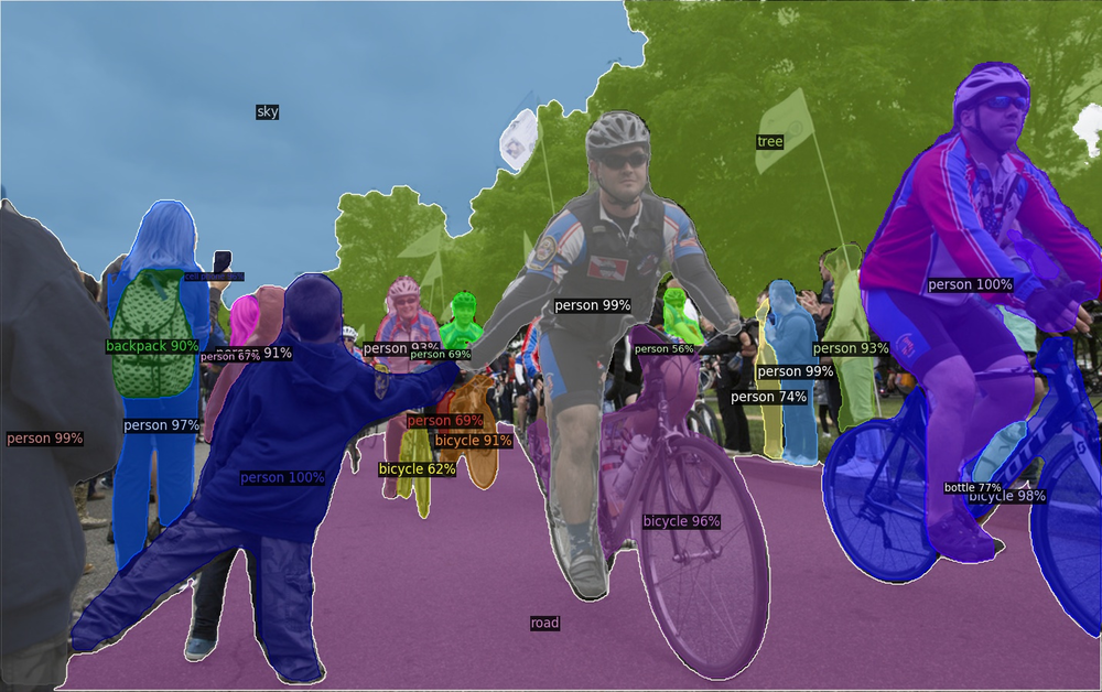
- Image segmentation CSAIL repo, detectron2
- Depth estimation Github
- 3D Pose estimation
- Generative Adversial Networks (e.g. NVlabs stylegan3), see also fakestylegan
- Speech synthesis/recognition (Ze, Senior, & Schuster, 2013), (Li et al., 2019)
- Automatic translation (Google Neural Machine Translation)
- Language models (BERT, GPT, chatGPT 175B) (Devlin, Chang, Lee, & Toutanova, 2019),(Brown et al., 2020)

See also Deep reinforcement learning : Atari / AlphaGO / AlphaStar / AlphaChem; Graph neural networks, etc..
Ressources
Books


People and conferences
Some of the major contributors to the field:
- N-2 : McCulloch/Pitts, Rumelhart, Rosenblatt, Hopfield,
- N-1 : Hinton, Bengio, LeCun, Schmidhuber
- N : Goodfellow, Dauphin, Graves, Sutskever, Karpathy, Krizevsky, Hochreiter
Some the most important conferences: NIPS/NeurIPS, ICLR, CVPR, (ICML, ICASSP, ..)
Online ressources :
- distill.pub, blog posts (e.g. pytorch.org blog),
- FastAI lectures, CS231n, MIT S191
- awesome deep learning, Awesome deep learning papers
Evaluation [1/2]
You will be evaluated by the participation to the Kaggle competition GeoLifeCLEF 2022 - LifeCLEF 2022 x FGVC9 on location-based species presence prediction.

Training: 1.663.996 observations covering 17.037 plants and animal species
Testing: one prediction every 10th days in 2017
Evaluation metric Top 30 error (lower is better)
Data: You can download them but they are all already available on the frontal and compute nodes of the DCE on /mounts/Datasets4/GeoLifeCLEF2022/
Some key points :
- long tailed distribution, large dataset (1 hour/epoch on a RTX 3090, Resnet50), image (rasters) + tabular data
- the challenge is over (best to beat 0.68472), an overview is available in (Joly et al., 2022) (see references.pdf)
- some litterature is available as some competitors described their solution, e.g. in the leaderboard
Definition
A neural network is a directed graph :
- nodes : computational units
- edges : weighted connections


There are two types of graphs :
- no cycle : feedforward neural network
- with at least one cycle : recurrent neural networks
But why do we care about convolutional neural networks with a softmax output, ReLu hiddden activations, cross entropy loss, batch normalization layers, trained with RMSprop with Nesterov momentum regularized with dropout exactly ?
Perceptron (Rosenblatt, 1958)
- Classification : given \((x_i, y_i) \in \mathbb{R}^n \times \{-1, 1\}\)
- Sensory - Associative - Response architecture, \(\phi_j(x)\) with \(\phi_0(x) = 1\)
- Algorithm and geometrical interpretation

Architecture of the classifier
Given fixed, predefined feature functions \(\phi_j\), with \(\phi_0(x) = 1, \forall x \in \mathbb{R}^n\), the perceptron classifies \(x\) as :
\[\begin{align} y &= g(w^T \Phi(x))\\ g(x) &= \begin{cases}-1 &\text{if }\quad x < 0 \\ +1 & \text{if }\quad x \geq 0 \end{cases} \end{align}\]
with \(\phi(x) \in \mathbb{R}^{n_a+1}\), \(\phi(x) = \begin{bmatrix} 1 \\ \phi_1(x) \\ \phi_2(x) \\ \vdots \end{bmatrix}\)
Geometrical interpretation : correct classification
Decision rule : \(y = g(w^T \Phi(x))\)
Algorithm:
\[\begin{align}
w = \begin{cases}
w &\text{ if the input is correctly classified}\\
w + \phi(x_i) &\text{ if the input is incorrectly classified as -1}\\
w - \phi(x_i) &\text{ if the input is incorrectly classified as +1}
\end{cases}
\end{align}\]

Geometrical interpretation : misclassification
Decision rule : \(y = g(w^T \Phi(x))\)
Algorithm:
\[\begin{align}
w = \begin{cases}
w &\text{ if the input is correctly classified}\\
w + \phi(x_i) &\text{ if the input is incorrectly classified as -1}\\
w - \phi(x_i) &\text{ if the input is incorrectly classified as +1}
\end{cases}
\end{align}\]

Geometrical interpretation : multiple samples
Decision rule : \(y = g(w^T \Phi(x))\)
The intersection of the valid halfspaces is called the cone of feasibility (it may be empty).
Consider two samples \(x_1, x_2\) with \(y_1=+1\), \(y_2=-1\)

Kernel perceptron
Any linear predictor involving only scalar products can be kernelized (kernel trick, cf SVM);
Decision rule : \(\mbox{sign}(<w, x>)\)
Given \(w(t) = w_0 + \sum_{i \in \mathcal{I}} y_i x_i\)
\[\begin{align*} <w,x> &= <w_0,x> + \sum_{i \in \mathcal{I}} y_i <x_i, x> \\ \Rightarrow k(w,x) &= k(w_0, x) + \sum_{i \in \mathcal{I}} y_i k(x_i, x) \end{align*}\]

Polynomial kernel of degree \(d=3\) :
\[k(x, y) = (1 + <x, y>)^3\]
Training set : 50 samples
Real risk : \(92\%\)
Code : https://github.com/rougier/ML-Recipes/blob/master/recipes/ANN/kernel-perceptron.py
Limits of linear classification
Perceptrons and logistic regression perform linear separation in a predefined, fixed feature space.

What about learning these features \(\phi_j(x)\)?