Historical perspective

• Hodgkin-Huxley (Hodgkin & Huxley, 1952) : giant squid axon
• Formal neuron (McCulloch & Pitts, 1943) : the community gets very excited
• Perceptron (Rosenblatt, 1958) : linear classifier
• AdaLinE (Widrow & Hoff, 1962) : linear regressor
• Minsky/Papert (Minksy & Papert, 1969) : first winter
• Convolutional Neural networks (Fukushima, 1980),(LeCun et al., 1989) : great !
• Multilayer Perceptron and backprop (Rumelhart, Hinton, & Williams, 1986) : great !

but it is hard to train (except the CNN) and the SVM comes in the play in the 1990s … : second winter

• 2006 : pretraining greatly helps
• 2012 : AlexNet on ImageNet (10% better on test than the 2nd)
• Now on : lot of SOTA neural networks

For an overview : (Schmidhuber, 2015)

Success stories

• Speech synthesis/recognition (Ze, Senior, & Schuster, 2013), (J. Li et al., 2019)
• Automatic translation (Google Neural Machine Translation)
• Language models (BERT, GPT) (Devlin, Chang, Lee, & Toutanova, 2019)

See also Deep reinforcement learning : Atari / AlphaGO / AlphaStar / AlphaChem; Graph neural networks, etc..

Why is deep learning working “now”

Some of the reasons of the current success :

• GPU (speed of processing) / Data (regularizing)
  
• theoretical understandings on the difficulty of training deep networks (from 2006)

Libraries allow to easily implement/test/deploy neural networks :

• Torch (Lua) / PyTorch(Python/C++), Caffe(C++/Python), Caffe2 (RIP 2018)
• Microsoft CNTK
• Google Tensorflow / Keras
• Theano/Lasagne (Python, RIP 2017)
• CNTK, Chainer, Matlab, Mathematica, ….

Ressources

Books

People and conferences

Some of the major contributors to the field:

• N-2 : McCulloch/Pitts, Rumelhart, Rosenblatt, Hopfield,
• N-1 : Hinton, Bengio, LeCun, Schmidhuber
  
• N : Goodfellow, Dauphin, Graves, Sutskever, Karpathy, Krizevsky, Hochreiter

Some the most important conferences: NIPS/NeurIPS, ICLR, (ICML, ICASSP, ..)
Online ressources :
- distill.pub, blog posts (e.g. pytorch.org blog),
- FastAI lectures, CS231n, MIT S191
- awesome deep learning, Awesome deep learning papers

Syllabus

Lecture 1/2 (08/02): Introduction, Linear networks, RBF
Lecture 3/4 (10/02): Feedforward networks, differential programming, initialization and gradient descent

2 : 17/02 1TP : 21/02 1TP : 28/02 2 CM : 07/03 2 CM : 14/03 1 TP : 21/03

Lecture 5 (17/02): Regularization, and Convolutional neural networks architectures
Lecture 6 (17/02-07/03) : Convolutional Neural Networks : applications

Lecture 7 (07/03-14/03): Recurrent neural networks : architectures
Lecture 8 (14/03): Recurrent neural networks : applications

Labworks : on our GPU clusters (1080, 2080 Ti, pytorch), in pairs, remotely with VNC.

Exam (22/03): 2h paper and pen exam

Definition

A neural network is a directed graph :

• nodes : computational units
• edges : weighted connections
  

There are two types of graphs :

• no cycle : feedforward neural network
  
• with at least one cycle : recurrent neural networks

Perceptron (Rosenblatt, 1958)

• Classification : given \((x_i, y_i) \in \mathbb{R}^n \times \{-1, 1\}\)
  
• Sensory - Associative - Response architecture, \(\phi_j(x)\) with \(\phi_0(x) = 1\)
  
• Algorithm and geometrical interpretation

Architecture of the classifier

Given fixed, predefined feature functions \(\phi_j\), with \(\phi_0(x) = 1, \forall x \in \mathbb{R}^n\), the perceptron classifies \(x\) as :

\[\begin{align} y &= g(w^T \Phi(x))\\ g(x) &= \begin{cases}-1 &\text{if }\quad x < 0 \\ +1 & \text{if }\quad x \geq 0 \end{cases} \end{align}\]

with \(\phi(x) \in \mathbb{R}^{n_a+1}\), \(\phi(x) = \begin{bmatrix} 1 \\ \phi_1(x) \\ \phi_2(x) \\ \vdots \end{bmatrix}\)

Online training algorithm

Given \((x_i, y_i)\), \(y_i \in \{-1,1\}\), the perceptron learning rule operates online: \[\begin{align} w = \begin{cases} w &\text{ if the input is correctly classified}\\ w + \phi(x_i) &\text{ if the input is incorrectly classified as -1}\\ w - \phi(x_i) &\text{ if the input is incorrectly classified as +1} \end{cases} \end{align}\]

Geometrical interpretation : correct classification

Decision rule : \(y = g(w^T \Phi(x))\)
Algorithm:
\[\begin{align} w = \begin{cases} w &\text{ if the input is correctly classified}\\ w + \phi(x_i) &\text{ if the input is incorrectly classified as -1}\\ w - \phi(x_i) &\text{ if the input is incorrectly classified as +1} \end{cases} \end{align}\]

Geometrical interpretation : misclassification

Decision rule : \(y = g(w^T \Phi(x))\)
Algorithm:
\[\begin{align} w = \begin{cases} w &\text{ if the input is correctly classified}\\ w + \phi(x_i) &\text{ if the input is incorrectly classified as -1}\\ w - \phi(x_i) &\text{ if the input is incorrectly classified as +1} \end{cases} \end{align}\]

Geometrical interpretation : multiple samples

Decision rule : \(y = g(w^T \Phi(x))\)

The intersection of the valid halfspaces is called the cone of feasibility (it may be empty).

Consider two samples \(x_1, x_2\) with \(y_1=+1\), \(y_2=-1\)

Toward a canonical learning rule

Given \((x_i, y_i)\), \(y_i \in \{-1,1\}\), the perceptron learning rule operates online: \[\begin{align} w = \begin{cases} w &\text{ if the input is correctly classified}\\ w + \phi(x_i) &\text{ if the input is incorrectly classified as -1}\\ w - \phi(x_i) &\text{ if the input is incorrectly classified as +1} \end{cases} \end{align}\]

Toward a canonical learning rule

Given \((x_i, y_i)\), \(y_i \in \{-1,1\}\), the perceptron learning rule operates online:

\[\begin{align*} w = \begin{cases} w &\text{ if } g(w^T\phi(x_i)) = y_i\\ w + y_i \phi(x_i) &\text{ if } g(w^T \phi(x_i)) \neq y_i \end{cases} \end{align*}\]

Perceptron convergence theorem

Definition (Linear separability)

A binary classification problem \((x_i, y_i) \in \mathbb{R}^d \times \{-1,1\}, i \in [1..N]\) is said to be linearly separable if there exists \(\textbf{w} \in \mathbb{R}^d\) such that~:

\[\begin{align*} \forall i, \mbox{sign}(\textbf{w}^T x_i) = y_i \end{align*}\]

with \(\forall x < 0, \mbox{sign}(x) = -1, \forall x \geq 0, \mbox{sign}(x) = +1\).

Theorem (Perceptron convergence theorem)

A classification problem \((x_i, y_i) \in \mathbb{R}^d \times \{-1,1\}, i \in [1..N]\) is linearly separable if and only if the perceptron learning rule converges to an optimal solution in a finite number of steps.

\(\Leftarrow\): easy; \(\Rightarrow\) : we upper/lower bound \(|w(t)|_2^2\)

Various facts

• \(w_t = w_0 + \sum_{i \in \mathcal{I}(t)} y_i \phi(x_i)\), with \(\mathcal{I}(t)\) the set of misclassified samples
  
• it minimizes a loss : \(J(w) = \frac{1}{N} \sum_i \max(0, -y_i w^T \phi(x_i))\)
  
• the solution can be written as

\[\begin{equation} w_t = w_0 + \sum_{i}\frac{1}{2} (y_i - \hat{y}_i) \phi(x_i) \end{equation}\]

\((y_i - \hat{y}_i)\) is the prediction error

Kernel perceptron

Any linear predictor involving only scalar products can be kernelized (kernel trick, cf SVM);

Decision rule : \(\mbox{sign}(<w, x>)\)

Given \(w(t) = w_0 + \sum_{i \in \mathcal{I}} y_i x_i\)

\[\begin{align*} <w,x> &= <w_0,x> + \sum_{i \in \mathcal{I}} y_i <x_i, x> \\ \Rightarrow k(w,x) &= k(w_0, x) + \sum_{i \in \mathcal{I}} y_i k(x_i, x) \end{align*}\]

Polynomial kernel of degree \(d=3\) :

\[k(x, y) = (1 + <x, y>)^3\]

Training set : 50 samples

Real risk : \(92\%\)

Code : https://github.com/rougier/ML-Recipes/blob/master/recipes/ANN/kernel-perceptron.py

Linear regression analytically

Problem : Given \((x_i, y_i)\), \(x_i\in\mathbb{R}^{n+1}, y_i \in \mathbb{R}\), minimize

\[ J(w) = \frac{1}{N} \sum_i ||y_i - w^T x_i||^2 \]

We assume that \(x_i[0] = 1 \forall i\) so that \(w[0]\) hosts the bias term.

Linear regression with stochastic gradient descent

Problem : Given \((x_i, y_i)\), \(x_i\in\mathbb{R}^{n+1}, y_i \in \mathbb{R}\), minimize

\[ J(w) = \frac{1}{N} \sum_i ||y_i - w^T x_i||^2 \]

We assume that \(x_i[0] = 1 \forall i\) so that \(w[0]\) hosts the bias term.

Batch gradient descent

\[J(w,x,y) = \frac{1}{N} \sum_{i=1}^N L(w,x_i,y_i)\] e.g. \(L(w,x_i,y_i) = ||y_i - w^T x_i||^2\)

Batch gradient descent

• compute the gradient of the loss \(J(w)\) over the whole training set

• performs one step in direction of \(-\nabla_w J(w,x,y)\) \[w_{t+1} = w_t - \epsilon_t \textcolor{red}{\nabla_w J(w,x,y)}\]

• \(\epsilon\) : learning rate

Stochastic gradient descent

\[J(w,x,y) = \frac{1}{N} \sum_{i=1}^N L(w,x_i,y_i)\] e.g. \(L(w,x_i,y_i) = ||y_i - w^T x_i||^2\)

Stochastic gradient descent (SGD)

• one sample at a time, noisy estimate of \(\nabla_w J\)

• performs one step in direction of \(-\nabla_w L(w,x_i,y_i)\) \[w_{t+1} = w_t - \epsilon_t \textcolor{red}{\nabla_w L(w,x_i,y_i)}\]

• faster to converge than gradient descent

Minibatch gradient descent

\[J(w,x,y) = \frac{1}{N} \sum_{i=1}^N L(w,x_i,y_i)\] e.g. \(L(w,x_i,y_i) = ||y_i - w^T x_i||^2\)

Minibatch

• noisy estimate of the true gradient with \(M\) samples (e.g. \(M=64, 128\)); \(M\) is the minibatch size
  
• Randomize \(\mathcal{J}\) with \(|\mathcal{J}| = M\), one set at a time

\[ w_{t+1} = w_t - \epsilon_t \textcolor{red}{\frac{1}{M} \sum_{j \in \mathcal{J}} \nabla_w L(w,x_j,y_j)} \]

• smoother estimate than SGD
• great for parallel architectures (GPU)

If the batch size is too large, there is a generalization gap (LeCun, Bottou, Orr, & Müller, 1998), maybe due to sharp minimum (Keskar, Mudigere, Nocedal, Smelyanskiy, & Tang, 2017); see also (Hoffer, Hubara, & Soudry, 2017)

Does it make sense to use gradient descent ?

Convex function A function \(f: \mathbb{R}^n \mapsto \mathbb{R}\) is convex :

1. \(\iff \forall x_1, x_2 \in \mathbb{R}^n, \forall t \in [0,1]\) \(f(t x_1 + (1-t)x_2) \leq t f(x_1) + (1-t) f(x_2)\)

2. with \(f\) twice diff.,
   \(\iff \forall x \in \mathbb{R}^n, H = \nabla^2 f(x)\) is positive semidefinite
   i.e. \(\forall x \in \mathbb{R}^n, x^T H x \geq 0\)

For a convex function \(f\), all local minima are global minima. Our losses are lower bounded, so these minima exist. Under mild conditions, gradient descent and stochastic gradient descent converge, typically \(\sum \epsilon_t =\infty, \sum \epsilon_t^2 < \infty\) (cf lectures on convex optimization).

Summary

Problem : Given \((x_i, y_i)\), \(x_i\in\mathbb{R}^{n+1}, y_i \in \mathbb{R}\)

• We assume that \(x[0] = 1\) to encompass the bias
  
• Linear model : \(\hat{y} = w^T x\)
  
• L2 loss : \(L(ŷ, y) = \|\hat{y} - y \|^2\)
• by gradient descent \[ \nabla_w L(w,x_i,y_i) = \frac{\partial L}{\partial \hat{y}} \frac{\partial \hat{y}}{\partial w} = -(y_i - \hat{y}_i) x_i \]

Other choices may also be considered (Huber loss, MAE, …).

Possibly regularized (but more on regularization latter).

Linear regression with L2 loss is convex

Indeed,

• Given \(x_i, y_i\), \(L(w) = \frac{1}{2}(w^T x_i - y_i)^2\) is convex:

\[ \begin{align*} \nabla_w L &= (w^T x_i - y_i) x_i\\ \nabla_w^2 L &= x_i x_i^T\\ \forall x \in \mathbb{R}^n x^T x_i x_i^T x &= (x_i^T x)^2 \geq 0 \end{align*} \]

• a non negative weighted sum of convex functions is convex

Maximum likelihood (binary classification)

Problem : Given \((x_i, y_i)\), \(x_i\in\mathbb{R}^{n}, y_i \in \{0, 1\}\)

Assume that \(P(y=1 | x) = p(x; w)\), parametrized by \(w\), and our samples to be independent, the conditional likelihood of the labels is:

\[ \mathcal{L}(w) = \prod_i P(y=y_i | x_i) = \prod_i p(x_i; w)^{y_i} (1- p(x_i; w))^{1-y_i} \]

With maximum likelihood estimation, we rather equivalently minimize the averaged negative log-likelihood :

\[ J(w) = -\frac{1}{N} \log(\mathcal{L}(w)) = \frac{1}{N} \sum_i -y_i\log(p(x_i; w))-(1-y_i)\log(1-p(x_i; w)) \]

Logistic regression (binary classification)

Problem : Given \((x_i, y_i)\), \(x_i\in\mathbb{R}^{n+1}, y_i \in \{0, 1\}\)

• Linear logit model : \(o(x) = w^Tx\) (we still assume \(x[0] = 1\) for the bias)

• Sigmoid transfer function : \(\hat{y}(x) = p(x; w) = \sigma(o(x)) = \sigma(w^T x)\)

  • \(\sigma(x) = \frac{1}{1 + \exp(-x)}\), \(\sigma(x) \in [0, 1]\)
    
  • \(\frac{d}{dx}\sigma(x) = \sigma(x) (1 - \sigma(x))\)

• Following maximum likelihood estimation, we minimize : \[ J(w) = \frac{1}{N} \sum_i -y_i\log(p(x_i; w))-(1-y_i)\log(1-p(x_i; w)) \]

• The loss \(L(\hat{y}, y) = -y \log(\hat{y}) - (1-y)\log(1 - \hat{y})\) is called the cross entropy loss, or negative log-likelihood

• The gradient of the cross entropy loss with \(\hat{y}(x) = \sigma(x)\) is : \[ \nabla_w L(w,x_i,y_i) = \frac{\partial L}{\partial \hat{y}} \frac{\partial \hat{y}}{\partial w} = -(y_i - \hat{y}_i) x_i \]

Logistic regression is convex

Indeed,

• Given \(x_i, y_i=1\), \(L_1(w) = -\log(\sigma(w^T x_i) = \log(1 + \exp(-w^Tx_i))\),
  \(\nabla_w L_1 = -(1 - \sigma(w^Tx_i)) x_i\)
  \(\nabla_w^2 L_1 = \underbrace{\sigma(w^T x_i) (1-\sigma(w^Tx_i))}_{>0} x_i x_i^T\)
• Given \(x_i, y_i=0\), \(L_2(w) = -\log(1-\sigma(w^T x_i))\)
  \(\nabla_w L_2 = \sigma(w^T x_i) x\)
  \(\nabla_w^2 L_2 = \underbrace{\sigma(w^T x_i) (1-\sigma(w^Tx_i))}_{>0} x_i x_i^T\)
• a non negative weighted sum of convex functions is convex

Do not use a L2 loss

Compute the gradient to see why

Take L2 loss \(L(\hat{y}, y) = \frac{1}{2}||\hat{y} - y||^2\)

• Take the “linear” model : \(\hat{y}_i = \sigma(w^T x_i)\)
  
• Check that \(\frac{d}{dx} \sigma(x) = \sigma(x) (1 - \sigma(x))\)
  
• Compute the gradient wrt \(w\):
  \[ \nabla_w L(w,x_i,y_i) = \frac{\partial L}{\partial \hat{y}} \frac{\partial \hat{y}}{\partial w} = (\hat{y}_i - y_i) \textcolor{red}{\sigma(w^T x_i) (1 - \sigma(w^T x_i))} x_i \]
• If \(x_i\) is strongly misclassified (e.g. \(y_i=1\), \(w^T x_i = -\infty\)). Then \(\sigma(w^T x_i) (1 - \sigma(w^T x_i)) \approx 0\), i.e. \(\nabla_w L(w,x_i,y_i) \approx 0\) \(\Rightarrow\) stepsize is very small while the sample is misclassified

With a cross entropy loss, \(\nabla_w L(w,x_i,y_i)\) is proportional to the error

Softmax regression (multiclass classification)

Problem : Given \((x_i, y_i)\), \(x_i\in\mathbb{R}^{n+1}, y_i \in [|0, K-1|]\)

Assume that \(P(y=c | x) = \frac{e^{w_c^T x}}{\sum_k e^{w_k^T x}}\), parametrized by \(w_0, w_1, w_2, ..\), and our samples to be independent, the conditional likelihood of the labels is:

\[ \mathcal{L}(w) = \prod_i P(y=y_i | x_i) \]

With maximum likelihood estimation, we rather equivalently minimize the averaged negative log-likelihood:

\[ J(w) = -\frac{1}{N} \log(\mathcal{L}(w)) = -\frac{1}{N} \sum_i \log(P(y=y_i | x_i)) \]

With a one-hot encoding of the target class (i.e. \(y_i = [0, ..., 0, 1, 0, .. ]\)), it can be written as :

\[ J(w) = -\frac{1}{N} \log(\mathcal{L}(w)) = -\frac{1}{N} \sum_i \sum_c y_c \log(P(y=c | x_i)) \]

Softmax regression (multiclass classification)

Problem : Given \((x_i, y_i)\), \(x_i\in\mathbb{R}^{n+1}, y_i \in [|0, K-1|]\)

• Linear models for each class \(o_j(x) = w_j^T x\) (we still assume \(x[0] = 1\))
  
• Softmax transfer function : \(P[y=j|x] = \hat{y}_j = \frac{\exp(o_j(x))}{\sum_k \exp(o_k(x))}\)
• Generalization of the sigmoid for a vectorial output
  
• Following maximum likelihood estimation, we minimize \[ J(w) = -\frac{1}{N} \log(\mathcal{L}(w)) = -\frac{1}{N} \sum_i \log(P(y=y_i | x_i)) \]
• The loss \(L(\hat{y}, y) = -\log(\hat{y}_y)\) is called the cross-entropy loss
• by gradient descent: \[\nabla_{w_j} L(w,x,y) = \sum_k \frac{\partial L}{\partial \hat{y}_k} \frac{\partial \hat{y}_k}{\partial w_j} = -(\delta_{j,y} - \hat{y}_j) x\]

Softmax regression is convex.

Numerical issues with the softmax and CE loss

Large exponentials

If you compute naïvely the softmax, you would have \(\exp(..)\) which is quickly large.

Fortunately:

\[ softmax(o_1, o_2, o_3, ..) = softmax(o_1 - o^\star, o_2 - o^\star, o_3-o^\star) = \frac{\exp(o_i - o^\star)}{\sum_j \exp(o_j - o^\star)} \]

You always compute \(\exp(z)\) with \(z \leq 0\).

Avoiding some exponentials with the log-sum-exp trick \(\log(\sum_j \exp(o_j)) = o^\star + \log(\sum_j \exp(o_j-o^\star))\)

You do not really need to compute the \(\log(\hat{y}_j) = \log(softmax_j(x)))\) since :

\[ \log(\hat{y}_i) = \log(\frac{\exp(o_i-o^\star)}{\sum_j \exp(o_j - o^\star)}) = o_i - o^\star - \log(\sum_j \exp(o_j - o^\star)) \]

In practice that explains why we use the Cross entropy loss with logits outputs rather than Softmax + Negative log likelihood or even LogSoftMax + NLLLoss (which does not have the log… yeah confusing…)

Limits of linear classification

Perceptrons and logistic regression perform linear separation in a predefined, fixed feature space.

What about learning these features \(\phi_j(x)\)?

Architecture (Broomhead & Lowe, 1988)

• RBFN are prototype based function approximator.
  
• specific architecture with a single layer of learnable feature vectors with “weights” (parameters) \((\mu_j, \sigma_j)_{j\in[0..N_a-1]}\)

\[ \begin{eqnarray*} \phi(x) = \begin{pmatrix} 1 \\ \exp{\frac{-||x-\mu_0||^2}{2\sigma_0^2}} \\ \vdots\\ \exp{\frac{-||x-\mu_{N_a-1}||^2}{2\sigma_{N_a-1}^2}} \\ \end{pmatrix} \end{eqnarray*} \]

Learning

• We know how to learn the weights \(w\) : minibatch gradient descent (or a variant thereof)

• What about the centers and variances ? (Schwenker, Kestler, & Palm, 2001)

  • place them uniformly, randomly, by vector quantization (K-means++(Arthur & Vassilvitskii, 2007), GNG (Fritzke, 1994))

  • two phases : fix the centers/variances, fit the weights

  • three phases : fix the centers/variances, fit the weights, fit everything (\(\nabla_{\mu} L, \nabla_{\sigma} L, \nabla_w L\))

Universal approximator

Theorem : Universal approximation (Park & Sandberg, 1991)

Denote \(\mathcal{S}\) the family of functions based on RBF in \(\mathbb{R}^d\): \[\mathcal{S} = \{g \in \mathbb{R}^d \to \mathbb{R}, g(x) = \sum_i w_i K(\frac{x-\mu_i}{\sigma}), w \in \mathbb{R}^N\}\] with \(K : \mathbb{R}^d \rightarrow \mathbb{R}\) continuous almost everywhere and \(\int_{\mathbb{R}^d}K(x)dx \neq 0\),
Then \(\mathcal{S}\) is dense in \(L^p(\mathbb{R})\) for every \(p \in [1, \infty)\)

In particular, it applies to the gaussian kernel introduced before.

Example

Architecture

Architecture

Vocabulary

• Depth : number of weight layers
• Width : number of units per layer
• Parameters : Weights and biases for every unit
• Skip layer connections can bypass layers
  
• one hidden transfer function \(f\), one task-specific output transfer function \(g\)

Hidden transfer function

• historically: hyperbolic tangent \(\tanh(x) = \frac{e^x - e^{-x}}{e^x + e^{-x}}\) or sigmoid \(\sigma(x) = \frac{1}{1 + \exp(-x)}\)
• now mainly Recitifed Linear Units (ReLu)(Nair & Hinton, 2010),(Krizhevsky et al., 2012) or variants : \[ \mbox{relu}(x) = \max(x, 0) \]

ReLu are more favorable for the gradient flow than the saturating functions (more on that latter when discussing computational graphs and gradient computation).

Some other recent hidden transfer functions

Output transfer function

Exactly as when we discussed about the RBF, this is task dependent.

Universal approximation

Any well behaved function can be arbitrarily approximated with a single layer FNN (Cybenko, 1989), (Hornik, 1991)

Intuition

• Transform the input with a linear transform \(y=w^Tx\)
  
• Take a sigmoid transfer function \(z = f(y) = \frac{1}{1+e^{-y}}\) : this is the output of the hidden layer
• combine multiple activities in the \(z-\)layer to build up gaussian like kernels

• weight such substractions and you are back to the RBF universal approximation theorem

Why do we bother about deep learning ?

• Single hidden layer FFN are universal approximators but the hidden layer can be arbitrarily large

• early theoretical results on logic gates circuits (Hastad, 1986). More recent works on ReLU FFN (Montufar, Pascanu, Cho, & Bengio, 2014)

Training : error backpropagation

Training is performed by gradient descent which was popularized by (Rumelhart et al., 1986) who called it error backpropagation (but (Werbos, 1981) already introduced the idea, see (Schmidhuber, 2015)).

Example on a regression problem

Overall steps :

0- Imports
1- Loading the data
2- Define the network
3- Define the loss, optimizer, callbacks, …
4- Iterate and monitor

Example on a regression problem

0- Imports

import torch
import torch.nn as nn
import torch.optim as optim

import sklearn
import sklearn.datasets

import tqdm

import matplotlib.pyplot as plt

1- Loading the data

# Load the data and build up our dataloader
data = sklearn.datasets.fetch_california_housing()
# X is (20640, 8), y is (20640, )
X, y = data.data, data.target

# At least normalize the input for an easier optimization
mean, std = X.mean(axis=0), X.std(axis=0)
X = (X - mean)/std

X_train = torch.tensor(X).float()
y_train = torch.tensor(y).float()

# A mapable dataset defines __len__ and __getitem__ (see also iterable datasets)
# it can also be an iterable dataset
train_dataset = torch.utils.data.TensorDataset(X_train, y_train)
# A dataloader will create the minibatches
train_dataloader = torch.utils.data.DataLoader(train_dataset,
                                               batch_size=64,
                                               shuffle=True,
                                               pin_memory=True)

Doc: Dataset, DataLoader. Pin memory
Iterating over train_dataloader gives a pair of tensors of shape \((64, 8)\) and \((64,)\).

Example on a regression problem

2- Define the network

if torch.cuda.is_available():
    device = torch.device('gpu')
else:
    device = torch.device('cpu')

# Build up the model
Nh = 64
model = nn.Sequential(
    nn.Linear(8, Nh), nn.ReLU(),
    nn.Linear(Nh, Nh), nn.ReLU(),
    nn.Linear(Nh, Nh), nn.ReLU(),
    nn.Linear(Nh, 1)
)

model.to(device)

Doc: Linear, Sequential

Example on a regression problem

3- Define the loss, optimizer, callbacks, …

# Define the loss
loss = nn.MSELoss()

# Define the gradient descent algorithm
optimizer = optim.Adam(model.parameters(),
                       lr=0.001)
scheduler = optim.lr_scheduler.StepLR(optimizer,
                                      step_size=10,
                                      gamma=0.5,
                                      verbose=True)

Doc: MSELoss, Adam, StepLR

Example on a regression problem

4- Iterate and monitor

for e in range(num_epochs):
    # Switch the network in train mode
    model.train()

    print(f"Epoch {e}")
    for X, y in tqdm.tqdm(train_dataloader):
        # Send the data to the GPU if necessary
        X, y = X.to(device), y.to(device)

        # Reset the gradient accumulator
        optimizer.zero_grad()

        # Forward pass
        y_pred = model(X).squeeze()
        loss_value = loss(y_pred, y)

        # Backward pass
        loss_value.backward()

        # Weight update
        optimizer.step()

    print(f"MSELoss on the training set : {mseloss(train_dataloader)}")

    # Update the learning rate after one epoch
    scheduler.step()

Evaluation

def mseloss(loader):
    # After every epoch, compute the risk
    # on the loader
    cum_loss = 0.0
    n_samples = 0
   
    # Switch the network in eval mode
    model.eval()

    with torch.no_grad():
        for X, y in tqdm.tqdm(loader):
            X, y = X.to(device), y.to(device)

            # Forward pass
            y_pred = model(X).squeeze()
            loss_value = loss(y_pred, y)

            # The loss is 'mean' reduced so be carefull when cumulating it
            cum_loss += loss_value * y_pred.size()[0]
            n_samples += y_pred.size()[0]
    return cum_loss/n_samples

Computational graph

A computational graph is a directed acyclic graph where nodes are :

• variables (weights, inputs, outputs, targets, …)
  
• operations (ReLu, Softmax, \(w^Tx + b\), losses, updates, ..)

Example graph for a linear regression \(\mathbb{R}^8 \mapsto \mathbb{R}\) with minibatch \((X, y)\)

\[ J = \frac{1}{M} \sum_{i=0}^{63} (w_1^T x_i + b_1 - y_i)^2 \]

Computational graph

Problem computing the partial derivatives with respect to the variables \(\frac{\partial J}{\partial var}\).

You just need to provide the local derivatives of the output w.r.t the inputs.

And then apply the chain rule.

ex : \(\frac{\partial J}{\partial w_1} \in \mathcal{M}_{1, 8}(\mathbb{R})\), assuming numerator layout

Computational graph : the chain rule

Numerator layout convention (otherwise, we transpose and reverse the jacobian product order):

The derivative of a scalar with respect to a vector is a row vector : \[ y \in \mathbb{R}, x \in \mathbb{R}^n, \frac{dy}{dx} \in \mathcal{M}_{1, n}(\mathbb{R}) \]

More generally, the derivative of a vector valued function \(y : \mathbb{R}^{n_x} \mapsto \mathbb{R}^{n_y}\) with respect to its input (the Jacobian) is a \(n_y \times n_x\) matrix :

\[ x \in \mathbb{R}^{n_x}, y(x) \in \mathbb{R}^{n_y}, \frac{dy}{dx}(x) = \begin{bmatrix} \frac{\partial y_1}{\partial x_1} & \frac{\partial y_1}{\partial x_2} & \cdots & \frac{\partial y_{1}}{\partial x_{n_x}} \\ \frac{\partial y_2}{\partial x_1} & \frac{\partial y_2}{\partial x_2} & \cdots & \frac{\partial y_{2}}{\partial x_{n_x}} \\ \vdots & \vdots & \ddots & \vdots \\ \frac{\partial y_{n_y}}{\partial x_1} & \frac{\partial y_{n_y}}{\partial x_2} & \cdots & \frac{\partial y_{n_y}}{\partial x_{n_x}} \end{bmatrix}(x) \]

Computational graph : the chain rule

For a (single-path) chain \(y_1 \rightarrow y_2 = f_1(y_1) \rightarrow y_3 = f_2(y_2) \cdots y_n = f_{n-1}(y_{n-1})\), of vector valued functions \(y_1 \in \mathbb{R}^{n_1}, y_2\in\mathbb{R}^{n_2}, \cdots y_n \in \mathbb{R}^{n_n}\),

\[ \frac{\partial y_n}{\partial y_1} = \frac{\partial y_n}{\partial y_{n-1}}\frac{\partial y_{n-1}}{\partial y_{n-2}}\cdots\frac{\partial y_2}{\partial y_1} \]

ex : \(\frac{\partial J}{\partial w_1} = \frac{\partial J}{\partial y_1} \frac{\partial y_1}{\partial w_1} = \frac{2}{M} (y_1-y)^T X \in \mathbb{R}^8\), assuming numerator layout

For matrix variables, we should be introducing tensors. See also this and this

The chain rule : multiple paths

The chain rule : multiples paths

But this can be computationally (too) expensive :

• there can be many paths you need to identify and sum over : L layers, N units, \(N^L\) paths
  
• and you must repeat the process for every variable w.r.t. which you want to differentiate
• some computations can be factored (e.g. \(\frac{\partial y_2}{\partial x}\), \(\frac{\partial y_1}{\partial x}\))

Automatic differentiation : forward mode

Let us be more efficient : forward mode differentiation

Idea: To compute \(\frac{\partial y}{\partial x}\), forward propagate \(\frac{\partial }{\partial x}\)
e.g. \(\frac{\partial y}{\partial x} = y_3 e^{y_1} \left[ w_2^T + y_2 w_1^T\right] + y_4 e^{y_2}\left[ w_1^T + y_1 w_2^T\right]\)

Welcome to the field of automatic differentiation (AD). For more, see (Griewank, 2012), (Griewank & Walther, 2008) (see also (Olah, 2015), (Paszke et al., 2017))

Automatic differentiation : reverse mode

Let us be (sometimes) even more efficient : reverse mode differentiation

Idea: To compute \(\frac{\partial y}{\partial x}\), backward propagate \(\frac{\partial y}{\partial }\) (compute the adjoint)
e.g. \(\frac{\partial y}{\partial x} = (y_4y_1e^{y_2} + y_3 e^{y_1})w_2^T + (y_3y_2e^{y_1} + y_4 e^{y_2})w_1^T\)

Gradient error backpropagation

In (Rumelhart et al., 1986), the algorithm was called “error backpropagation” : why ?

Suppose a 2-layer multi-layer feedforward network and propagating one sample, with a scalar loss : \[ L = g( y_i, \begin{bmatrix} & & \\ & W_2 (n_2 \times n_1) & \\ & & \end{bmatrix} f( \begin{bmatrix} & & \\ & W_1 (n_1 \times n_x) & \\ & & \end{bmatrix} \begin{bmatrix} \\ x_i \\ \phantom{} \end{bmatrix} )) \in \mathbb{R} \]

\(g\) could be a squared loss for regression (with \(n_2=1\)), or CrossEntropyLoss (with logits and \(n_2=n_{class}\)) for multiclass classification.

We denote \(z_1 = W_1 x_i, z_2 = W_2 f(z_1)\) and \(\delta_i = \frac{\partial L}{\partial z_i} \in \mathbb{R}^{n_i}\). Then : \[ \begin{align} \delta_2 &= \frac{\partial L}{\partial z_2} = \frac{\partial g(x_1, x_2)}{\partial x_2}(y_i, z_2) \\ \delta_1 &= \frac{\partial L}{\partial z_1} = \frac{\partial L}{\partial z_2} \frac{\partial z_2}{\partial z_1} = \begin{bmatrix} & & \delta_2 & & \end{bmatrix} \begin{bmatrix} & & \\ & W_2(n_2 \times n_1) & \\ & & \phantom{}\end{bmatrix} \text{diag}(f'(z_1)) \end{align} \] The errors of \(\delta_2\) are integrated back through the weight matrix that was used for the forward pass. (See also (Nielsen, 2015), chap 2).

Gradient descent in deep learning

• Evaluation of the outputs : forward propagation / forward pass
• Evaluation of the gradient : reverse-mode differentiation / backward pass

Gradient descent in practice

• The deep learning frameworks all compute the backward pass automatically.

optimizer = optim.Adam(model.parameters())

for e in range(epochs):
    for X,y in train_dataloader:
        optimizer.zero_grad()
        ...
        loss.backward()
        optimizer.step()

import torch.autograd.Function as Function

class MyFunction(Function):

    @staticmethod
    def forward(ctx, input, ..): 
        ...

    @staticmethod
    def backward(ctx, grad_output):
        ...

The way toward differentiable programming

The computational graph is a central notion in modern neural networks/deep learning. Broaden the scope with differential programming.

In the recent years, “fancier” differentiable blocks others than \(f(W f(W..))\), and that are dynamically built (eager mode vs static graph).

Does it make sense to use gradient descent ?

Indeed :

• we cannot do better than a local minima
• neural networks lead to non convex optimization. For example, consider a 2-layer FFN :

But empirically, most local minima are close (in performance) to the global minimum, especially with large/deep networks. See (Dauphin et al., 2014), (Pascanu, Dauphin, Ganguli, & Bengio, 2014), (Choromanska, Henaff, Mathieu, Arous, & LeCun, 2015). Saddle points seem to be more critical.

First order methods : Minibatch stochastic gradient descent

Algorithm

• Start at \(\theta_0\)
• for every minibatch : \[ \begin{align*} \theta(t+1) &= \theta(t) - \epsilon \nabla_\theta L(\theta(t))\\ L(\theta) &= \frac{1}{M} \sum_i J(\theta, x_i, y_i) \end{align*} \]

Rationale (Taylor expansion) : \(L(\theta_{t+1}) \approx L(\theta_{t}) + (\theta_{t+1} - \theta_{t})^T \nabla_{\theta} L(\theta_{t})\)

The choice of the batch size :

• Stochastic gradient descent (small minibatch, \(M=1\)) : noisy estimate, not GPU friendly
• Batch Gradient descent (\(M=N\)) : More GPU friendly. But more prone to bad generalization (generalization gap) and to local minima (Keskar et al., 2017). Roughly speaking, we should avoid sharp minima.

The optimization may converge slowly or even diverge if the learning rate \(\epsilon\) is not appropriate.

Choosing a learning rate

Bengio: “The optimal learning rate is usually close to the largest learning rate that does not cause divergence of the training criterion” (Bengio, 2012)

Karpathy “\(0.0003\) is the best learning rate for Adam, hands down.” (Twitter, 2016)

(Note: Adam will be discussed in few slides)

See also :
- Practical Recommendations for gradient-based training of deep architectures (Bengio, 2012)
- Efficient Backprop (LeCun et al., 1998)

Example regression problem

Setup

• \(N=30\) samples generated with : \[ y = 3 x + 2 + \mathcal{U}(-0.1, 0.1) \]
• Model : \(f_\theta(x) = \theta^T\begin{bmatrix} 1 \\ x\end{bmatrix}\),
• L2 loss : \(L(y_i, f_{\theta}(x_i)) = (y_i - f_{\theta}(x_i))^2\)

Example using SGD

Parameters : \(\epsilon=0.005\), \(\theta_0 = \begin{bmatrix} 10 \\ 5\end{bmatrix}\)

Converges to \(\theta_{\infty} = \begin{bmatrix} 1.9882 \\ 2.9975\end{bmatrix}\)

First order methods : momentum

Algorithm : Let us damp the oscillations with a low pass on \(\nabla_{\theta}\)

• Start at \(\theta_0\), \(v_0 = 0\)
• for every minibatch : \[ \begin{align*} v(t+1) &= \mu v(t) - \epsilon \nabla_{\theta} J(\theta(t))\\ \theta(t+1) &= \theta(t) + v(t+1) \end{align*} \]

Usually \(\mu \approx 0.9\) or \(0.99\).

• as an exponential moving average, it low pass filters and therefore dampen oscillations along fast varying dimensions
• it can accelerate (increase the learning rate) in constant directions (or low curvature).
  If \(\nabla_{\theta} J = g\), \(v(0) = 0\) \[ v(t) = -\epsilon g \sum_{i=0}^{t-1} \mu^i = -\epsilon g \frac{1-\mu^{t}}{1-\mu} \]

See also distill.pub. Note the frameworks may implement subtle variations.

Example using SGD with momentum

Parameters : \(\epsilon=0.005\), \(\mu=0.6\), \(\theta_0 = \begin{bmatrix} 10 \\ 5\end{bmatrix}\)

Converges to \(\theta_{\infty} = \begin{bmatrix} 1.9837 \\ 2.9933\end{bmatrix}\)

First order methods : Nesterov momentum

Idea Look ahead to potentially correct the update. Based on Nesterov Accelerated Gradient. Formulation of (Sutskever et al., 2013)

Algorithm

• Start at \(\theta_0\)
• for every minibatch : \[ \begin{align*} \overline{\theta}(t) &= \theta(t) + \mu v(t)\\ v(t+1) &= \mu v(t) - \epsilon \nabla_{\theta}J(\overline{\theta}(t))\\ \theta(t+1) &= \theta(t) + v(t+1) \end{align*} \]

Example using SGD with Nesterov momentum

Parameters : \(\epsilon=0.005\), \(\mu=0.8\), \(\theta_0 = \begin{bmatrix} 10 \\ 5\end{bmatrix}\)

Converges to \(\theta_{\infty} = \begin{bmatrix} 1.9738 \\ 2.9914\end{bmatrix}\)

Comparison of the 1st order methods

On our simple regression problem

First order : adaptive learning rate

You should always adapt your learning rate with a learning rate scheduler

• Linear decrease from \(\epsilon_0\) downto \(\epsilon_f\)
• halve the learning rate when the validation error stops improving
• halve the learning rate on a fixed schedule (every \(50th\) epochs)

Adaptive first order : adaptive learning rate

Some more recent approaches are changing the picture of “decreasing learning rate” (“Robbins Monro conditions”)

See (Smith, 2018), The 1cycle policy - S. Gugger

Stochastic Gradient Descent with Warm Restart (Loshchilov & Hutter, 2017)

The improved performances may be linked to reaching flatter minimums (i.e. with predictions less sensitive than sharper minimums). The models reached before the warm restarts can be averaged (see Snapshot ensemble).

It seems also that initial large learning rates tend to lead to better models on the long run (Y. Li et al., 2019)

Adaptive first order : Adagrad

Adagrad Adaptive Gradient (Duchi, Hazan, & Singer, 2011)

• Accumulate the square of the gradient \[ r(t+1) = r(t) + \nabla_{\theta}J(\theta(t)) \odot \nabla_{\theta}J(\theta(t))\\ \]
• Scale individually the learning rates \[ \theta(t+1) = \theta(t) - \frac{\epsilon}{\delta + \sqrt{r(t+1)}} \odot \nabla_{\theta}J(\theta(t)) \]

The \(\sqrt{.}\) is experimentally critical ; \(\delta \approx [1e-8, 1e-4]\) for numerical stability.

Small gradients \(\rightarrow\) bigger learning rate for moving fast along flat directions
Big gradients \(\rightarrow\) smaller learning rate to calm down on high curvature.

Adaptive first order : RMSprop

RMSprop Hinton(unpublished, Coursera)

Idea: we should be using an exponential moving average when accumulating the gradient.

• Accumulate the square of the gradient \[ r(t+1) = \rho r(t) + (1-\rho)\nabla_{\theta}J(\theta(t)) \odot \nabla_{\theta}J(\theta(t))\\ \]
• Scale individually the learning rates \[ \theta(t+1) = \theta(t) - \frac{\epsilon}{\delta + \sqrt{r(t+1)}} \odot \nabla_{\theta}J(\theta(t)) \] \(\rho \approx 0.9\)

Adaptive first order : ADAM

Adaptive Moments (ADAM) (Kingma & Ba, 2015)

• Like momentum and RMSprop, store running averages of past gradients : \[ \begin{align*} m(t+1) &= \beta_1 m(t) + (1-\beta_1)\nabla_{\theta}J(\theta(t)\\ v(t+1) &= \beta_2 v(t) + (1-\beta_2)\nabla_{\theta}J(\theta(t)\odot \nabla_{\theta}J(\theta(t) \end{align*} \] \(m(t)\) and \(v(t)\) are the first moment and second (uncentered) moments of \(\nabla_{\theta} J\). They are bias corrected \(\hat{m}(t)\), \(\hat{v}(t)\) and then :

\[ \theta(t+1) = \theta(t) - \frac{\epsilon}{\delta + \sqrt{\hat{v}(t+1)}} \hat{m}(t+1) \]

First order : to sum up

(Goodfellow, Bengio, & Courville, 2016) There is currently no consensus[…] no single best algorithm has emerged[…]the most popular and actively in use include SGD,SGD with momentum, RMSprop, RMSprop with momentum, Adadelta and Adam.

See also Chap. 8 of (Goodfellow et al., 2016)

A glimpse into second order methods

Rationale : \[ J(\theta) \approx J(\theta_0) + (\theta - \theta_0)^T \nabla_{\theta}J(\theta_0) + \frac{1}{2}(\theta - \theta_0)^T \nabla^2_{\theta} J(\theta_0) (\theta - \theta_0) \] with \(H = \nabla^2J\) the Hessian matrix, a \(n_\theta \times n_\theta\) matrix hosting the second derivatives of \(J\).

The second derivates are much more noisy than the first derivative (gradient), a larger batch size is usually required to prevent instabilities.

• Conjugate gradient : using line search (or hessian) along \(\nabla_{\theta}J(\theta_k)\)
  
• Newton : never use except if you want to find critical points (Dauphin et al., 2014). Solves above for \(\theta\) and find \(\nabla_\theta^2J(\theta_0) . (\theta - \theta_0) = -\nabla_\theta J(\theta_0)\)
• Quasi Newton : BFGS (approximating \(H^{-1}\)), L-BFGS, and saddle-free versions (Dauphin et al., 2014).

The starting point is important : XOR

XOR is easy right ?

• Model : 2-4-1, Sigmoid activations (great!); 17 parameters
• Init : \(\mathcal{U}(−10, 10)\), bias=0 (hum hum)
• Loss : Binary cross entropy (great!)
• Optimizer : SGD ( = 0.1, momentum=0.99 )

But it fails miserably (6/20 fails). Tmax=1000

The starting point is important : XOR

XOR is easy right ?

• Model : 2-4-1, Sigmoid activations (great!); 17 parameters

• Loss : Binary cross entropy (great!)
• Optimizer : SGD ( = 0.1, momentum=0.99 )

Now it is better (0/20 fails). Tmax=1000

Pretraining

Historically, training deep FNN was known to be hard, i.e. bad generalization errors.

The starting point of a gradient descent has a dramatic impact :

• neural history compressors (Schmidhuber, 1992)
• competitive learning (Maclin & Shavlik, 1995)
• unsupervised pretraining based on Boltzman machines (Hinton, 2006)
• unsupervised pretraining based on auto-encoders (Bengio, Lamblin, Popovici, & Larochelle, 2006)

Pretraining is no more used (because of xxRelu, Initialization schemes, ..)

Standardizing your inputs

Gradient descent converges faster if your data are normalized and decorrelated. Denote by \(x_i \in \mathbb{R}^d\) your input data, \(\hat{x}_i\) its normalized.

• Min-max scaling \[ \forall i,j \hat{x}_{i,j} = \frac{x_{i,j} - \min_k x_{k,j}}{\max_k x_{k,j} - \min_k x_{k,j} + \epsilon} \]

• Z-score normalization (goal: \(\hat{\mu}_j = 0, \hat{\sigma}_j = 1\)) \[ \forall i,j, \hat{x}_{i,j} = \frac{x_{i,j} - \mu_j}{\sigma_j + \epsilon} \]

• ZCA whitening (goal: \(\hat{\mu}_j = 0, \hat{\sigma}_j = 1\), \(\frac{1}{n-1} \hat{X} \hat{X}^T = I\))

\[ \hat{X} = W X, W = \frac{1}{\sqrt{n-1}} (XX^T)^{-1/2} \]

Z-score normalization / Standardizing the inputs

Remember our linear regression : \(y = 3x+2+\mathcal{U}(-0.1, 0.1)\), L2 loss, 30 1D samples

General strategy

• A good initialization should break the symmetry : constant initialization schemes make units learning all the same thing

• A good initialization should start optimization in a region of low capacity : linear neural network

• A good initialization scheme should preserve the distribution of the activations and gradients : exploding/vanishing gradients

The exploding and vanishing gradient problem

The Fundamental Deep Learning Problem first observed by (Josef Hochreiter, 1991) for RNN, the gradient can either vanish or explode, especially in deep networks (RNN are very deep).

• Remember that the backpropagated gradient involves : \[ \frac{\partial J}{\partial x_l} = \frac{\partial J}{\partial y_L} W_L f'(y_l) W_{L-1} f'(y_{l-1}) \cdots \] with \(y_l = W_l x_l + b, x_l = f(y_{l-1})\).

• We see a pattern like \((W.f')^L\) which can diverge or vanish for large \(L\).

• especially, with the sigmoid :\(f' < 1\).

With a ReLu, the positive part has \(f' = 1\).

Preventing vanishing/exploding gradient

• We must ensure a good flow of gradient :
  • using appropriate transfer functions ReLu, PreLu, etc..
  • using architectural elements :
    • ResNet (CNN) : shortcurt connections
    • LSTM (RNN): constant error caroussel
• We can prevent exploding gradient by clipping (Pascanu, Mikolov, & Bengio, 2013)

LeCun Initialization

In (LeCun et al., 1998), Y. LeCun provided some guidelines on the design:

Aim Initialize the weights/biases to keep \(f\) in its linear part through multiple layers:

Xavier (Glorot) Initialization

Idea we must preserve the same distribution along the forward and backward pass (Glorot & Bengio, 2010).

This prevents:

• the saturation of saturating transfer functions (e.g. tanh, sigmoid)
• vanishing/exploding gradient

Glorot (Xavier) initialization scheme for a feedforward network \(f(W_{n}..f(W^1f(W_0 x+b_0)+b_1)...+b_n)\) with layer sizes \(n_i\):

• the input dimensions should be centered, normalized, uncorrelated
• symmetric activation function, with \(f'(0) = 1\) (e.g. \(f(x)=\tanh(x), f(x)=4(\frac{1}{1+e^{-x}}-0.5)\))

Assuming the linear regime \(f'() = 1\) of the network : \[ \begin{align*} \mbox{Forward propagation variance constraint :} \forall i, fan_{in_i} \sigma^2_{W_i} &= 1\\ \mbox{Backward propagation variance constraint :} \forall i, fan_{out_i} \sigma^2_{W_i} &= 1 \end{align*} \] Compromise : \(\forall i, \frac{1}{\sigma^2_{W_i}} = \frac{fan_{in} + fan_{out}}{2}\)
- Glorot (Xavier) uniform : \(\mathcal{U}(-\frac{\sqrt{6}}{\sqrt{fan_{in}+fan_{out}}}, \frac{\sqrt{6}}{\sqrt{fan_{in}+fan_{out}}})\), b=0
- Glorot (Xavier) normal : \(\mathcal{N}(0, \frac{\sqrt{2}}{\sqrt{fan_{in}+fan_{out}}})\), b=0

He Initialization

Idea we must preserve the same distribution along the forward and backward pass for rectifiers (He et al., 2015). For a feedforward network \(f(W_{n}..f(W^1f(W_0 x+b_0)+b_1)...+b_n)\) with layer sizes \(n_i\):

• the input dimensions should be centered, normalized, uncorrelated
• ReLu activation \(f(x) = \max(x, 0)\)
• weights initialized with symmetric distribution, zero mean \(\mu_{w_l} = 0\), independently. Bias set to \(b=0\)
• the components of \(x_l\) are assumed i.i.d.; Note they are not centered (because of ReLu) \[ \begin{align*} \mathbf{y}_l &= \begin{bmatrix} \vdots \\ y_l \\ \vdots\end{bmatrix} = W_l \mathbf{x}_l + \mathbf{b} = W_l f(\mathbf{y}_{l-1}) + \mathbf{b}\\ \mu_{y_l} &= E[\sum_i w_{l,i}x_{l,i}] = \mu_{w_l}\sum_i \mu_{x_{l,i}} = 0\\ \sigma^2_{y_l} &= n_l\sigma^2_{w_l x_l} = n_l \mu_{w_l^2} \mu_{x_l^2} = n_l \sigma^2_{w_l} \mu_{x_l^2} (\mbox{because $\mu_{w_l} = 0$})\\ \mu_{x_l^2} &= \int_{y_{l-1}} \max(0, y_{l-1})^2dp_{y_{l-1}} = \frac{1}{2} \mu_{y_{l-1}^2} =\frac{1}{2} \sigma^2_{y_{l-1}} (\mbox{$\mu_{y_{l-1}}=0$ and $y_{l-1}$ has symmetric distrib.}) \end{align*} \]

So, \(\sigma^2_{y_l} = \frac{1}{2}n_l \sigma^2_{w_l} \sigma^2_{y_{l-1}}\). To preserve the variance, we must guarantee \(\frac{1}{2} n_l \sigma^2_{w_l} = 1\).

We used : if \(X\) and \(Y\) are independent : \(\sigma^2_{X.Y} = \mu_{X^2}\mu_{Y^2} - \mu_X^2 \mu_Y^2\)

He initialization

Idea we must preserve the same distribution along the forward and backward pass for rectifiers (He et al., 2015). For a feedforward network \(f(W_{n}..f(W^1f(W_0 x+b_0)+b_1)...+b_n)\) with layer sizes \(n_i\):

• the input dimensions should be centered, normalized, uncorrelated
• ReLu activation \(f(x) = \max(x, 0)\)
• weights initialized with symmetric distribution, zero mean \(\mu_{w_l} = 0\), independently. Bias set to \(b=0\)
• the components of \(x_l\) are assumed i.i.d.; Note they are not centered (because of ReLu)

\[ \begin{align*} \mbox{Forward propagation variance constraint :} \forall i, \frac{1}{2}fan_{in_i} \sigma^2_{W_i} &= 1\\ \mbox{Backward propagation variance constraint :} \forall i, \frac{1}{2}fan_{out_i} \sigma^2_{W_i} &= 1 \end{align*} \]

He suggests to use either one or the other, e.g. \(\sigma^2_{W_i} = \frac{2}{fan_{in}}\)
- He uniform : \(\mathcal{U}(-\frac{\sqrt{6}}{\sqrt{fan_{in}}}, \frac{\sqrt{6}}{\sqrt{fan_{in}}})\), b=0
- He normal : \(\mathcal{N}(0, \frac{\sqrt{2}}{\sqrt{fan_{in}}})\), b=0

Note: for PreLu : \(\frac{1}{2} (1 + a^2) fan_{in} \sigma^2_{W_i} = 1\)

Weight initialization in practice (PyTorch)

By default, the parameters are initialized randomly. e.g. in torch.nn.Linear :

class Linear(torch.nn.Module):
    def __init__(self):
        ...
        self.reset_parameters()
    
    def reset_parameters(self) -> None:
        # Setting a=sqrt(5) in kaiming_uniform is the same as initializing with
        # uniform(-1/sqrt(in_features), 1/sqrt(in_features)). For details, see
        # https://github.com/pytorch/pytorch/issues/57109
        torch.nn.init.kaiming_uniform_(self.weight, a=math.sqrt(5))
        fan_in, _ = torch.init.calculate_fan_in_and_fan_out(self.weight)
        bound = 1/math.sqrt(fan_in)
        init.uniform_(self.bias, -bound, bound)

import torch.nn.init as init

class MyModel(torch.nn.Module):
    def __init__(self):
        super(MyModel, self).__init__()
        self.classifier =  nn.Sequential(
            *linear_relu(input_size, 256),
            *linear_relu(256, 256),
            nn.Linear(256, num_classes)
        )
        self.init()

    def init(self):
        @torch.no_grad()
        def finit(m):
            if type(m) == nn.Linear:
                init.kaiming_uniform_(m.weight,
                                      a=0,
                                      mode='fan_in',
                                      nonlinearity='relu')
                m.bias.fill_(0.0)
        self.apply(finit)

def linear_relu(dim_in, dim_out):
    return [nn.Linear(dim_in, dim_out),
            nn.ReLU(inplace=True)]

Internal covariate shift

(Ioffe & Szegedy, 2015) observed the change in distribution of network activations due to the change in network parameters during training.

Experiment 3 fully connected layers (100 units), sigmoid, softmax output, MNIST dataset

Batch Normalization

Idea standardize the activations of every layers to keep the same distributions during training (Ioffe & Szegedy, 2015)

• The gradient must be aware of this normalization, otherwise may get parameter explosion (see (Ioffe & Szegedy, 2015)) \(\rightarrow\) we need a differentiable normalization layer

• introduces a differentiable Batch Normalization layer : \[ z = g(W x + b) \rightarrow z = g(BN(W x)) \]

Batch normalization

During training

• put BN layers everywhere along the network, after the linear layer, before the ReLus
  
• evaluate the statistics \(\mu, \sigma\) over the minibatches
• update an exponential moving average of the mean \(\mu_{\mathcal{B}}\) and variance \(\sigma^2_{\mathcal{B}}\)

During inference (test) :

• use the running average as the statistics to standardize : this is now just a fixed affine transform.

model = MyModel()  # a pytorch nn.Module
# For training
model.train()
# For testing
model.test()

L2 penalty

Add a L2 penalty on the weights, \(\alpha > 0\)

\[ \begin{align*} J(\theta) &= L(\theta) + \frac{\alpha}{2} \|\theta\|^2_2 = L(\theta) + \frac{\alpha}{2}\theta^T \theta\\ \nabla_\theta J &= \nabla_\theta L + \alpha \theta\\ \theta &\leftarrow \theta - \epsilon \nabla_\theta J = (1 - \alpha \epsilon) \theta - \epsilon \nabla_\theta L \end{align*} \] Called L2 regularization, Tikhonov regularization, weight decay

Example RBF, 1 kernel per sample, \(N=30\), noisy inputs,

See chap 7 of (Goodfellow et al., 2016) for a geometrical interpretation

Intuition : for linear layers, the gradient of the function equals the weights. Small weights \(\rightarrow\) small gradient \(\rightarrow\) smooth function.

L2 penalty

In theory, regularizing the bias will cause underfitting

Example

\[ \begin{align*} J(w, b) &= \frac{1}{N} \sum_{i=1}^N \| y_i - b - w^T x_i\|_2^2\\ \nabla_b J(w,b) &\implies b = (\frac{1}{N} \sum_i y_i) - w^T (\frac{1}{N} \sum_i x_i) \end{align*} \]

If your data are centered (as they should), the optimal bias is the mean of the targets.

L1 penalty

Add a L1 penalty to the weights : \[ \begin{align*} J(\theta) &= L(\theta) + \alpha \|\theta\|_1 = L(\theta) + \alpha \sum_i |\theta_i|\\ \nabla_\theta J &= \nabla_\theta L + \alpha \mbox{sign}(\theta) \end{align*} \]

Example RBF, 1 kernel per sample, \(N=30\), noisy inputs,

See chap 7 of (Goodfellow et al., 2016) for a mathematical explanation in a specific case. Sparsity used for feature selection with LASSO (filter/wrapper/embedded).

Dropout

Introduced in (Srivastava, Hinton, Krizhevsky, Sutskever, & Salakhutdinov, 2014):

Idea 1 : preventing co-adaptation. A pattern is robust by itself not because of others doing part of the job.
Idea 2 : average of all the sub-networks (ensemble learning)

How :

• for every minibatch, zeroes hidden and input activations with probability \(p\) (\(p=0.5\) for hidden, \(p=0.2\) for input). At test time, multiply every activations by \(p\)

• “Inverted” dropout : multiply the kept activations by \(p\) at train time. At test time, just do a normal forward pass.

Dropout

• Usually, after all fully connected layers (p=0.5) and input layer
• less usual on convolutional layers (because these are already regularized)

Can be interpreted as if training/averaging all the possible subnetworks.

L1/L2/Dropout in pytorch

L1/L2

class MyModel(nn.Module):
    def __init__(..., l2_reg, ..):
        self.lin1 = nn.Linear(784, 256)
        self.lin2 = nn.Linear(256, 256)
        self.l2_reg = l2_reg

    def penalty(self):
        return l2_reg * (self.lin1.weight.norm(2) + ...) 

def train():
    ...
    optimizer.zero_grad()
    loss.backward()
    model.penalty().backward()

Dropout

import torch.nn as nn

class MyModel(nn.Module):
    def __init__(self, ..):
        self.classifier = nn.Sequential(
            *dropout_linear_relu(784, 128, 0.5),
            *dropout_linear_relu(128, 256, 0.5),
            nn.Linear(256, num_classes)
        )

def dropout_linear_relu(dim_in, dim_out, p_zeroed):
    return [nn.Dropout(p_zeroed),
            nn.Linear(dim_in, dim_out),
            nn.ReLU(inplace=True)]

Early stopping

Split your data in three sets :

• training set : for training ..
  
• validation set: for choosing the hyperparameters (learning rates, number of layers, layer size, momentum, …)
  
• test set : for estimation the generalization error

Everything can be placed in a cross validation loop.

Early stopping is about keeping the model with the lowest validation loss.

# Training over an epoch
for X, y in tqdm.tqdm(train_dataloader):
    X, y = X.to(device), y.to(device)
    ...
    optimizer.step()
# Model checkpoint
val_loss = test(model, valid_loader)
if val_loss < best_val_loss:
    torch.save(model.state_dict(), filepath)

Data, data, we need data !

The best regularizer you may find is data. The more you have, the better you learn.

• you can use pretrained models on some tasks as an initialization for learning your task (but may fail due to domain shift) : check the Pytorch Hub

• you can use unlabeled data for pretraining your networks (as done in 2006s) with auto-encoders / RBM : unsupervised/semi-supervised learning

• you can apply random transformations to your data : dataset augmentation, see for example alubmentations.ai

Label smoothing

Introduced in (Szegedy, Vanhoucke, Ioffe, Shlens, & Wojna, 2015) in the context of Convolutional Neural Networks.

Idea : Preventing the network to be over confident on its predictions on the training set.

Recipe : in a \(k\)-class problem, instead of using hard targets \(\in \{0, 1\}\), use soft targets \(\in \{\frac{\alpha}{k}, 1-\alpha\frac{k-1}{k}\}\) (weighted average between the hard targets and uniform target). \(\alpha \approx 0.1\).

See also (Müller, Kornblith, & Hinton, 2020) for several experiments.

Extracting features with convolutions

From data that have a spatial structure (locally correlated), features can be extracted with convolutions.

On Images

That also makes sense for temporal series that have a structure in time.

A convolution as a sparse matrix multiply

What is a convolution : Example in 2D

Composition to learn higher level features

Local features can be combined to learn higher level features.

Let us build a house detector

Architecture

Ideas Using the structure of the inputs to limit the number of parameters without limiting the expressiveness of the network

• For inputs with spatial (or temporal) correlations, features can be extracted with convolutions of local kernels

• A convolution can be seen as a fully connected layer with :
  • a lot of weights set exactly to \(0\)
  • a lot of weights shared across positions

\(\rightarrow\) strongly regularized !

Vanilla CNN of LeCun

The architecture of LeNet-5 (LeCun et al., 1989), let’s call it the Vanilla CNN

CNN Vocabulary

We work with 4D tensors for 2D images, 3D tensors for nD temporal series (e.g. multiple simultaneous recordings), 2D tensors for 1D temporal series

In Pytorch, the tensors follow the Batch-Channel-Height-Width (BCHW, channel-first) convention. Other frameworks, like TensorFlow or CNTK, use BHWC (channel-last).

CNN in practice

Pytorch code for implementing a CNN : Conv1D Conv2D, MaxPool1D MaxPool2D, AveragePooling, etc…

conv_model  = nn.Sequential(
    *conv_relu_maxpool(cin=3, cout=32,
                       csize=3, cstride=1, cpad=1,
                       msize=2, mstride=2, mpad=0),
    *conv_relu_maxpool(cin=3, cout=64,
                       csize=3, cstride=1, cpad=1,
                       msize=2, mstride=2, mpad=0), 
)

def conv_relu_maxpool(cin, cout, csize, cstride, cpad, msize, mstride, mpad):
    return [nn.Conv2d(cin, cout, csize, cstride, cpad),
            nn.ReLU(inplace=True),
            nn.MaxPool2d(msize, mstride, mpad)
            ]

fc_model = nn.Sequential(
    *linear_relu(output_size, 256),
    nn.Linear(256, num_classes)
)

dummy_output = conv_model(torch.zeros((1, 3, height, width)))
output_size = np.prod(dummy_output.shape[1:] )

CNN in practice

All of these should fit into a nn.Module subclass :

class MyModel(torch.nn.Module):
    def __init__(self, ....):
        super(MyModel, self).__init__()
        self.conv_model = nn.Sequential(...)
        output_size = ...
        self.fc_model = nn.Sequential(...)

    def forward(self, inputs):
        conv_features = self.conv_model(inputs)
        conv_features = conv_features.view(inputs.shape[0], -1)
        return self.fc_model(conv_features)

You can also use the recently introduced nn.Flatten layer.

Transposed convolution

Given two 1D-vectors \(x_1, k\), say \(k = [c, b, a]\) \[ y_1 = (x_1 * k) = \begin{bmatrix} b & c & 0 & 0 & \cdots & 0 & 0 \\ a & b & c & 0 & \cdots & 0 & 0 \\ 0 & a & b & c & \cdots & 0 & 0 \\ 0 & 0 & a & b & \cdots & 0 & 0\\ \vdots & \vdots & \vdots & \vdots & \vdots & \vdots & \vdots\\ 0 & 0 & 0 & 0 & \cdots & b & c \\ 0 & 0 & 0 & 0 & \cdots & a & b \\ \end{bmatrix} . \begin{bmatrix} \\ x_1 \\ \phantom{}\end{bmatrix} = W_k x_1 \]

If we compute the gradient of the loss, in denominator layout: \[ \frac{\partial L}{\partial x_1} = \frac{\partial y_1}{\partial x_1}\frac{\partial L}{\partial y_1} = W_k^T \frac{\partial L}{\partial y_1} \]

Hence, it is coined the term transposed convolution or backward convolution. This will pop up again when speaking about deconvolution.

Multicolumn CDNN

Introduced in (Ciresan, Meier, & Schmidhuber, 2012), ensemble of CNNs trained with dataset augmentation

SuperVision

Introduced in (Krizhevsky et al., 2012), the “spark” giving birth to the revival of neural networks.

Supervision

The first layer learned to extract meaningful features

ZFNet

ILSVRC’13 winner. Introduced in (Zeiler & Fergus, 2014)

• Introduced visualization techniques to inspect which features are learned.

• Ablation studies on AlexNet : the FC layers are not that important

• Introduced the idea of supervised pretraining (pretraining on ImageNet, finetune the softmax for Caltech-101, Caltech-256, Pascal 2012)

• SGD minibatch(128), momentum(0.9), learning rate (0.01) manual schedule,

Deconvnet computes approximately the gradient of the loss w.r.t. the input (Simonyan, Vedaldi, & Zisserman, 2014). It differs in the way the ReLu is integrated.

VGG

ILSVRC’14 1st runner up. Introduced by (Simonyan & Zisserman, 2015).

• 16 layers : 13 convolutive, 3 fully connected
  
• Only \(3\times3\) convolution, \(2\times2\) pooling
• Stacked \(3\times3\) convolutions \(\equiv\) \(5\times5\) convolution receptive field with less parameters
  • If \(c_{in}=K, c_{out}=K\), \(5\times5\) convolution \(\rightarrow\) \(25K^2\) parameters
    
  • If \(c_{in}=K, c_{out}=K\), 2 stacked \(3\times3\) convolution \(\rightarrow\) \(18K^2\) parameters
    
• 140 million parameters, batch size(256), Momentum(0.9), Weight decay(\(0.0005\)), Dropout(0.5) in FC, learning rate(\(0.01\)) divided \(3\) times by \(10\)
• Initialization of \(B,C,D,E\) from trained \(A\). Init of \(A\) random \(\mathcal{N}(0, 10^{-2}), b=0\). Noticed (Glorot & Bengio, 2010) after submission.
• can cope with variable input size changing the FC layers to conv \(7\times 7\), conv\(1\times1\).

Striving for simplicity

Introduced in (Springenberg, Dosovitskiy, Brox, & Riedmiller, 2015).

• uses only convolutions, with various strides, no max pooling
• introduces “guided backpropagation” visualization

GoogLeNet (inception v1)

ILSVR’14 winner. Introduced by (Szegedy et al., 2014).

Idea Multi-scale feature detection and dimensionality reduction

• 22 layers, \(6.8\)M parameters
• trained in parallel , asynchronous SGD, momentum(0.9), learning rate schedule (\(4\%\) every 8 epochs)
• at test : polyak average and ensemble of \(7\) models
  
• auxiliary heads to mitigate vanishing gradient

Residual Networks (ResNet)

ILSVRC’15 winner. Introduced in (He et al., 2016a)

Residual Networks (ResNet)

Variations around skip layer connections

Highway Networks (Srivastava, Greff, & Schmidhuber, 2015)

• Uses “gates” (as in LSTM, see lectures on RNN) :
  • Transform gate \(T(x) = \sigma(W_T x + b_T)\)
    
  • Carry gate \(C(x) = \sigma(f_c(x))\)

\[ y = T(x).H(x) + C(x).x \]

DenseNets

Other networks

Fitnet [Romero(2015)], Wideresnet(2017), Mobilenetv1, v2, v3 [Howard(2019)] : searching for the best architecture, EfficientNet (Tan & Le, 2020)

See also :

• Papers with code
  
• SOTA bench

Number of filters

You should increase the number of filters throughout the network :

• the first layer extracts low level features
• the higher layers compose on the lower layer dictionary of features

Examples :

• LeNet-5 (1998) : \(6 5\times5\), \(16 5\times5\)
  
• AlexNet (2012) : \(96 11\times11\), \(256 5\times5\), \(2\times(384 3\times3)\), \(256 3\times3\)
  
• VGG (2014) : \(64-128-256-512\), all \(3\times 3\)
  
• ResNet (2015) : \(64-128-256-512\), all \(3\times 3\)
• Inception (2015) : \(32-64-80-192-288-768-1280-2048\), \(1\times1, 3\times3, '5\times5'\)

EfficientNet (Tan & Le, 2020) studies the scaling strategies of conv. models.

Effective receptive field (1/3)

Effective receptive field (2/3)

Effective receptive field (3/3)

A-trou convolutions

Your effective receptive field can grow faster with a-trou convolutions (or dilated convolutions) (Yu & Koltun, 2016):

Illustrations from this guide on conv arithmetic. The Conv2D object’s constructor accepts a dilation argument.

Stacking and factorizing small kernels

Introduced in Inception v3 (Szegedy et al., 2015)

\(n\) input filters,\(\alpha n\) output filters :

• \((\alpha n, 5\times5)\) conv : \(25 \alpha n^2\) params
• \((\sqrt{\alpha}n,3\times3)\)- \((\alpha n, 3\times3)\) : \(9\sqrt{\alpha}n^2+9\sqrt{\alpha}\alpha n^2\) params;

\(\alpha=2 \Rightarrow -24\%\) (\(\sqrt{\alpha}\) is critical!)

\(n\) input filters,\(\alpha n\) output filters :

• \((\alpha n, 3\times3)\) conv : \(9 \alpha n^2\) params
• \((\sqrt{\alpha}n, 1\times3)\) - \((\alpha n, 3\times1)\) : \(3\sqrt{\alpha}n^2 + 3\alpha \sqrt{\alpha}n^2\) params

\(\alpha=2 \Rightarrow -30\%\)

See also the recent work on “Rethinking Model scaling for convolutional neural networks” (Tan & Le, 2020)

Depthwise separabable convolutions

Inception and Xception, Mobilnets. It separates :

• feature extraction in each channel, in space : depthwise convolution
• feature combination between channels : pointwise convolution \(1\times1\)

Multi-scale feature extraction

See also the Feature Pyramid Networks for multi-scale features.

Dimensionality reduction

Trainable non-linear transformation of the channels. Network in network (Lin, Chen, & Yan, 2014)

Easing the gradient flow

You can check the norm of the gradient w.r.t. the first layers’ parameters to diagnose vanishing gradients

• Shortcut connections (e.g. ResNet, DenseNet, Highway)

• auxiliary heads (e.g. GoogleNet)

Do we need max pooling ?

Recent architectures remove the max pooling layers and replace them by conv(stride=2) for downsampling

Model and weight averaging

All the competitors in ImageNet do perform model averaging.

Model averaging

Weight averaging

If you worry about the increased computational complexity, see knowledge distillation (Hinton, Vinyals, & Dean, 2015) : training a light model with the soft targets (vs. the labels, i.e. the hard targets) of a computationally intensive one.

Using pre-trained models

All the frameworks provide you with a model zoo of pre-trained networks. E.g. in PyTorch, for image classification. You can cut the head and finetune the softmax only.

import torchvision.models as models

resnet18 = models.resnet18(pretrained=True)
alexnet = models.alexnet(pretrained=True)
vgg16 = models.vgg16(pretrained=True)
inception = models.inception_v3(pretrained=True)
googlenet = models.googlenet(pretrained=True)
mobilenet = models.mobilenet_v2(pretrained=True)
resnext50_32x4d = models.resnext50_32x4d(pretrained=True)
[...]

normalize = transforms.Normalize(mean=[0.485, 0.456, 0.406],
                                 std=[0.229, 0.224, 0.225])

Dataset augmentation

You can oversample around your training samples by applying transforms on the inputs that make predictable changes on the targets.

• color jittering, translations, reflections, rotations, PCA, …

Libraries for augmentation : albumentations, imgaug

See also mixup: Beyond empirical risk minimization

CIFAR-100 dataset

• The CIFAR-100 dataset is made of \(100\) classes with \(600\) images per class.
  
• The images are \(32\times 32\) RGB

• The training set has \(500\times 100\) images, and the test set has \(100 \times 100\) images.

Model architecture and optimization setup

Number of parameters: \(\simeq 2M\)
Time per epoch (1080Ti) : 17s. , 42min training time

If applied, only the weights of the convolution and linear layers are regularized (not the bias, nor the coefficients of the Batch Norm)

Baseline

No regularization (either L2, Dropout, Label smoothing, data augmentation), No BatchNorm

With BatchNorm

With batchnorm after every convolution (Note it is also regularizing the network)

With data augmentation

With dataset augmentation (HFlip, Scale, Trans)

With regularization

With regularization : L2 (0.0025), Dropout(0.5), Label smoothing(0.1)

Problem statement

Given :

• images \(x_i\),
  
• targets \(y_i\) which contains objects bounding boxes and labels

Examples from ImageNet (see here)

Bounding boxes given, in the datasets (the predictor parametrization may differ), by : \([x, y, w, h]\), \([x_{min},y_{min},x_{max},y_{max}]\), …

Datasets : Coco, ImageNet, Open Images Dataset

Recent survey : Object detection in 20 years: a survey

Open image evaluation:

• uses a variant of VOC 2010. more details here

A first step: object localization

Suppose you have a single object to detect, can you localize it into the image ?

RCNN

How can we proceed with multiple objects ? (Girshick, Donahue, Darrell, & Malik, 2014) proposed to :

• use selective search for proposing bounding boxes
• to classify with a SVM from the features extracted by a pretrained DNN.
  
• to optimize localization with linear bbox adaptors

Revolution in the object detection community (vs. “traditional” HOG like features).

Drawback :

• external algorithm (not in the computational graph, not trainable)
• one forward pass per bounding box proposal (\(\sim 2K\) or so) \(\rightarrow\) training and test are slow (\(47 s.\) per image with VGG16)

Fast RCNN

Introduced in (Girshick, 2015). Idea:

• just one forward pass
• cropping the convolutional feature maps (e.g. \((1, 512, H/16, W/16)\) conv5 of VGG16)
• max-pool the variable sized crop to a fixed-sized (e.g. \(7 \times 7\)) vector before dense layers: ROI pooling

Drawbacks:

• external algorithm for ROI proposals: not trainable and slow
• ROIs are snapped to the grid (see here) \(\rightarrow\) ROI align

Faster RCNN : 2-stages trained end-to-end

Introduced in (Ren, He, Girshick, & Sun, 2016). The first end-to-end trainable network. Introducing the Region Proposal Network (RPN). A RPN is a sliding Conv(\(3\times3\)) - Conv(\(1\times1\), k + 4k) network (see here). It also introduces anchor boxes of predefined aspect ratios learned by vector quantization.

Check the paper for a lot of quantitative results. Small objects may not have a lot of features.

FPN

Introduced in (Lin et al., 2017)

Upsampling is performed by using nearest neighbors.

For object detection, a RPN is run on every scale of the pyramid \(P_2, P_3, P_4, P_5\).

ROIPooling/Align is fed with the feature map at a scale depending on ROI size. Large ROI on small/coarse feature maps, Small ROI on large/fine feature maps

You Only Look Once (Yolo v1,v2,v3) (1/2)

The first one-stage detector. Introduced in (Redmon, Divvala, Girshick, & Farhadi, 2016). It outputs:

• \(B\) bounding boxes \((x, y, w, h, conf)\) for each cell of a \(S\times S\) grid
• the probabilities over the \(K\) classes
• the output volume is \((5\times B+K)\times(S\times S)\) in YoloV1, then \((5+K)\times B \times (S\times S)\) from v2

Bounding box encoding:

In YoLo v3, the network is Feature Pyramid Network (FPN) like with a downsampling and an upsampling paths, with predictions at 3 stages.

You Only Look Once (Yolo v1,v2,v3) (2/2)

The loss is multi-task with :

• a term for the regression of the transformation of the anchor boxes
• a term for detecting the presence of an object
• a term for the (possibly multi) labelling of the boxes

\[\begin{align*} \mathcal{L} &= \lambda_{coord} \sum_{i=0}^{S^2}\sum_{j=0}^{B} \mathbb{1}_{ij}^{obj} [(t_x-t_x^*)^2+(t_y-t_y^*)^2+(t_w-t_w^*)^2+(t_h-t_h^*)^2] \\ & -\sum_{i=0}^{S^2} \sum_{j=0}^{B} BCE(\mathbb{1}_{ij}^{obj}, \mbox{has_obj}_{ij}) \\ & -\sum_{i=0}^{S^2} \sum_{j=0}^{B} \sum_{k=0}^{K} BCE(\mbox{has_class}_{ijk}, p_{ijk}) \end{align*}\]

Non maximum suppression (NMS)

The object detectors may output multiple overlapping bounding box for the same object

NMS algorithm :

• order the bounding boxes by decreasing confidence
  
• for every rank, remove every bounding box, of lower rank, with IoU higher than a threshold

NMS may suppress one of two “overlapped” objects. It hard resets the scores of overlapping bboxes.

SoftNMS (Bodla, Singh, Chellappa, & Davis, 2017):

• order the bounding boxes by decreasing confidence
  
• for every rank, scale the confidence of the bounding boxes of lower rank bboxes (rather than setting to 0)

Problem statement

Given an image,

Semantic segmentation : predict the class of every single pixel. We also call dense prediction/dense labelling.

Example image from MS Coco

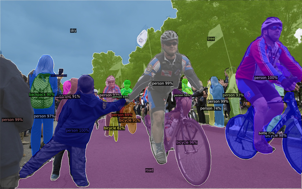
Instance segmentation : classify all the pixels belonging to the same countable objects

Example image from MS Coco

More recently, panoptic segmentation refers to instance segmentation for countable objects (e.g. people, animals, tools) and semantic segmentation for amorphous regions (grass, sky, road).

Metrics : see Coco panotpic evaluation

Some example networks : PSP-Net, U-Net, Dilated Net, ParseNet, DeepLab, Mask RCNN, …

Other CNN related problems we did not discuss

• Super resolution :
  • Learn to upscale an image
  • example networks : SRCNN, FSRCNN, VDSR, ESPCN, RED-Net

• Graph convolutions :

  • Learn to aggregate features on graph which are structures of arbitrary sizes and arbitrary branching factor
  • example networks : Weisfeilher lehman, see pytorch geometric, AlphaChem, ..

• Processing 3D point clouds :

  • unstructured sparse irregular 3D data
  • example networks : PointNet

Spatialising the time : TDNN

Time delay neural networks as introduced in (Waibel, Hanazawa, Hinton, Shikano, & Lang, 1989) spatializes the time:

Architecture of a RNN

Introduced by (Elman, 1990).

Weight matrices :

• \(W^{in}\) input to hidden
  
• \(W^h\) hidden to hidden
• \(W^{out}\) hidden to output
• \(W^{back}\) outputs to hidden

\[ \begin{align*} h(t) &= f(W^{in} x(t) + W^{h} h(t-1) + W^{back} y(t-1) + b_h)\\ y(t) &= g(W^{out} h(t) + b_y) \end{align*} \]

The hidden to hidden weight matrix \(W_{h}\) is repeatedly applied.

Named Elman networks if \(W^{back} = 0\), and Jordan networks if \(W^h = 0\). Elman networks with a random fixed \(W^h\) are called Echo State networks.

Many to One, One to Many, Many to Many

The inputs and outputs can be of variable (\(1 \rightarrow T_x\), \(1 \rightarrow T_y\)) and arbitrary sizes (\(T_x \neq T_y\)).

• Many to one example : language model, sentiment analysis : multiclass sequence classification \(T_y=1\):

  • \(['this', 'movie', 'was', 'fantastic'] \mapsto 1\)
  • \(['you', 'should', 'not', 'spend', 'even', 'a', 'single', 'penny', 'watching', 'this', 'movie'] \mapsto 0\)

• Many to many example : Neural Machine Translation

  • What is the most likely EN translation of “La croissance économique s’est ralentie ces dernières années.” : “Economic growth has slowed down in recent years.”

• One to many example: image captioning, language model with probabilistic sampling

Training with (truncated)-BPTT

Idea: unfold in time the computational graph and perform reverse mode differentiation (Werbos, 1990).

You must be training on truncated series to prevent a computational burden.

You can also perform forward mode differentiation (Real time recurrent learning RTTL (Williams & Peng, 1990)) with online adaptation as the inputs/targets comes in but this is computationally expensive.

Training a RNN can be hard

Unrolled in time, RNN appears as very deep networks \(\rightarrow\) vanishing/exploding gradient

• Initialization strategies :

  • LSTM : high forget bias to favor a remember by default (Gers, Schmidhuber, & Cummins, 2000)
  • orthogonal weight initialization (Henaff, Szlam, & LeCun, 2016), to keep the hidden activities normalized \(\|Wh\|_2^2 = h^T W^T W h = h^T h = \|h\|_2^2\), see also (Arjovsky, Shah, & Bengio, 2016)
  • identity recurrent weight initialization to favor a copy as-is by default for RNN (Le, Jaitly, & Hinton, 2015)

Long-Short Term memory (LSTM)

RNNs have difficulties learning long range dependencies. The LSTM (Hochreiter & Schmidhuber, 1997) introduces memory cells to address that problem.

Peepholes may connect the \(c_t\) to their gates.

Equations:

\[ \begin{eqnarray*} I_t &=& \sigma(W^x_i x_t + W^h_i h_{t-1} + b_i) &\in [0,1], \mbox{Input gate}\\ F_t &=& \sigma(W^x_f x_t + W^h_f h_{t-1} + b_f)&\in [0,1], \mbox{Forget gate}\\ O_t &=& \sigma(W^x_o x_t + W^h_o h_{t-1} + b_o) &\in [0,1], \mbox{Output gate}\\ n_t &=& \tanh(W^x_n x_t + W^h_n h_{t-1} + b_z)& \mbox{unit's input}\\ c_t &=& F_t \odot c_{t-1} + I_t \odot n_t& \mbox{cell update}\\ h_t &=& O_t \odot \tanh(c_t) & \mbox{unit's output} \end{eqnarray*} \] The next layers integrate what is exposed by the cells, i.e. the unit’s output \(h_t\), not \(c_t\).

If \(F_t=1, I_t=0\), the cell state \(c_t\) is unmodified. This is called the constant error carrousel.

Gated Recurrent Units (GRU)

The GRU is introduced as an alternative, simpler model than LSTM. Introduced in (Cho et al., 2014).

Equations:

\[ \begin{eqnarray*} R_t &=& \sigma(W^x_i x_t + W^h_i h_{t-1} + b_i) \mbox{ Reset gate}\\ Z_t &=& \sigma(W^x_z x_t + W^h_z h_{t-1} + b_z) \mbox{ Update gate}\\ n_t &=& \tanh(W^x_{n} x_t + b_{nx} + R_t \odot (W^h_nh_{t-1}+b_{nh}))\\ h_t &=& Z_t \odot h_{t-1} + (1-Z_t) \odot n_t \end{eqnarray*} \]

If \(Z_{t} = 1\), the cell state \(h_t\) is not modified. If \(Z_t = 0\) and \(R_t=1\), it is updated in one step.

Compared to LSTM, a GRU cell :

• unconditionally exposes its hidden state (there is no private cell state \(c_t\))
  
• the hidden state is reset by getting \(R_t=0\)

Bidirectional RNN/LSTM/GRU

Idea Both past and future contexts can sometimes be required for classification at the current time step; e.g. when you speak, past and future phonemes influence the way you pronounce the current one. Introduced in (Schuster & Paliwal, 1997})

Deep RNNs

While RNN are fundamentally deep neural networks, they can still benefit from being stacked : this allows the layers to operate at increasing time scales. The lower layers can change their content at a higher rate than the higher layers.

• (Graves et al., 2013): Phoneme classification with stacked bidirectionnal LSTMs

• (Sutskever, Vinyals, & Le, 2014) : Machine translation with stacked unidirectionnal LSTMs (Seq2Seq)

In a stacked RNN, you can concatenate consecutive hidden states before feeding in the next RNN layer, e.g. Listen, Attend and Spell encoder (\(\rightarrow\) downscale time)

Other variants for introducing depth in RNN is explored in (Pascanu et al., 2014). For example, the transition function from \(h_{t-1}\) to \(h_t\) is not deep, even in stacked RNNs but is deep in DT-RNN.

Defining RNN in PyTorch

Stacked bidirectional LSTM, documentation

with discrete inputs (words, characters, …) of the same time length, one prediction per time step.

import torch
import torch.nn as nn

seq_len = 51
batch_size = 32
vocab_size = 10
embedding_dim = 128
hidden_size = 256

rnn_model = nn.Sequential(
    nn.Embedding(num_embeddings=vocab_size,
                 embedding_dim=embedding_dim),
    nn.LSTM(input_size=embedding_dim,
            hidden_size=hidden_size,
            num_layers=3,
            bidirectional=True)
)
out_model = nn.Sequential(
    nn.Linear(2*hidden_size, 10)
)

# Forward propagation
# An embedding layer takes as input a LongTensor
rand_input = torch.randint(low=0, high=vocab_size,
                           size=(seq_len, batch_size))

# out_rnn is (T, B, num_hidden)
# state_n is the state of the last hidden layer
out_rnn, state_n = rnn_model(rand_input)

# out is (T, B, num_out)
out = out_model(out_rnn)

Digging into pytorch code

How do you know how to access these weights ? See the doc

Note several redundant biases \(b_{i.}\) and \(b_{h.}\) (for CuDNN compatibility).

Custom initialization

Task: initialize in the “Learning to forget” regime of (Gers et al., 2000)

        
num_layers=3

rnn = nn.LSTM(input_size=embedding_dim,
              hidden_size=hidden_size,
              num_layers=num_layers,
              bidirectional=True)

# Initialize to high forget gate bias
with torch.no_grad():
    for i in range(num_layers):
        forw_bias = getattr(rnn, f'bias_ih_l{i}').chunk(4, dim=0)[1]
        forw_bias.fill_(1)
        rev_bias = getattr(rnn, f'bias_ih_l{i}_reverse').chunk(4, dim=0)[1]
        rev_bias.fill_(1)

The ordering of the weights/biases are inputg/forgetg/cell/outputg.

Character level language model (Char-RNN)

Problem given fixed length chunks of sentences, predict the next word/character : \(p(x_T | x_0, x_1, ..., x_{T-1})\)

Many to many during training (teacher forcing (Williams & Peng, 1990)) but many to one for inference.

A language model can be used, e.g., to constrain the decoding of a network outputting sentences (e.g. in speech-to-text or captioning tasks)

See also The unreasonnable effectiveness of recurrent neural networks and (Sutskever, Martens, & Hinton, 2011).

Training and sampling from the character RNN

Example on “Les fabulistes”

• Vocabulary of 105 elements : {‘\t’: 0, ‘\n’: 1, ’ ‘: 2,’!‘: 3,’“‘: 4, "’”: 5, ‘(’: 6, ‘)’: 7, ‘*’: 8, ‘+’: 9, ‘,’: 10, ‘-’: 11, ‘.’: 12, ‘/’: 13, ‘0’: 14, ‘1’: 15, ‘4’: 16, ‘5’: 17, ‘6’: 18, ‘8’: 19, ‘9’: 20, ‘:’: 21, ‘;’: 22, ‘<’: 23, ‘>’: 24, ‘?’: 25, ‘A’: 26, ‘B’: 27, ‘C’: 28, ‘D’: 29, ‘E’: 30, ‘F’: 31, ‘G’: 32, ‘H’: 33, ‘I’: 34, ‘J’: 35, ‘L’: 36, ‘M’: 37, ‘N’: 38, ‘O’: 39, ‘P’: 40, ‘Q’: 41, ‘R’: 42, ‘S’: 43, ‘T’: 44, ‘U’: 45, ‘V’: 46, ‘W’: 47, ‘X’: 48, ‘Y’: 49, ‘Z’: 50, ‘\[’: 51, …}

Sampling from the character RNN

• After \(30\) epochs, validation loss of \(1.45\) and validation accuracy of \(56\%\).

• To sample from the language model, you can provide it with some context sentence, e.g.
  [‘L’, ‘A’, ’ ‘, ’G’, ‘R’,‘E’,‘N’,‘O’,‘U’, ‘I’, ‘L’, ‘L’, ‘E’, ’ ’]

Note the upper case after the line breaks, the uppercase title, the quite existing words. The text does not make much sense but it is generated character by character !

More on language modeling (metrics, models, …) in the Deep NLP lecture of Joel Legrand.

Image captioning

Problem Given an image, generate a textual description of it.

Example datasets : Coco captions, Flickr8k, Flickr30k

Some of the first entries : (Vinyals, Toshev, Bengio, & Erhan, 2015), (Xu et al., 2016)

Difficulty: object detection with their relationship

Show and tell

Idea Use a pre-trained CNN for image embedding plugged into a RNN for generating (decoding) the sequence of words. Introduced in (Vinyals et al., 2015).

Learn a model maximizing :

\[ p(S_0S_1S_2..S_T | I, \theta) = p(S_0|I, \theta)\prod_{j>0}^{T} p(S_j|S_0S_1...S_{j-1}, I, \theta) \]

i.e. minimizing \(-\log(p(S_0S_1S_2..S_T | I, \theta)) = -\sum_j \log(p(S_j|S_0...S_{j-1}, I, \theta))\)

Inspired by the Seq2Seq approach successful in machine translation (more on this later), they proposed an encoder-decoder model to translate an image to a sentence

Show and tell

Show attend and tell

Idea Allow the RNN to filter out/focus on CNN features during generation using an attention mechanism (Bahdanau, Cho, & Bengio, 2015). Introduced in (Xu et al., 2016). Link to theano source code

Show attend and tell

Where is the problem

Problem In tasks such as Machine Translation (MT) or Automatic Speech Recognition (ASR), input sequences get mapped to output sequences, both can be of arbitrary sizes.

Machine translation :

The proposal will not now be implemented

Les propositions ne seront pas mises en application maintenant

Automatic speech recognition

The alignment can be difficult to explicit. Contrary to the language model, we may not know easily when to output what.

Encoder / Decoder architectures

Idea Encode/Compress the input sequence to a hidden state and decode/decompress the output sequence from there. Introduced in (Cho et al., 2014) for ranking translations and (Sutskever et al., 2014) for generating translations (NMT).

Architecture :

• 4 layers LSTM(\(1000\), \(\mathcal{U}(-0.08, 0.08)\)), Embeddings(\(1000\))
• Vocabularies (in:\(160.000\), out:\(80.000\))
• SGD\((0.7\)), halved every half epoch after 5 epochs. Trained for \(7.5\) epochs. Batch(\(128\))
• gradient clipping \(5\)
• \(10\) days on \(8\) GPUs

The input sentence is fed in reverse order.

Beam search decoding. Teacher forcing for training but see also Scheduled sampling or Professor Forcing.

See Cho’s blog post. See this implementation in pytorch

Decoding with beam search

To get the most likely translation, you need to estimate

\[ p(y | x) = p(y_0|x, \theta) \prod_t p(y_t | y_0...y_{t-1} x \theta) \]

But the probability distribution over the labels is dependent on the previously generated label (which feeds the input for the next step) \(\rightarrow\) approximate search by maintaining a set of \(B\) candidates.

See also the modified beam search scoring of GNMT (Wu et al., 2016).

Connectionist Temporal Classification (CTC)

Idea For problems with the output sequence length \(T_y\) is smaller than the input sequence \(T_x\), allow a blank character. Introduced in (Graves, Fernández, Gomez, & Schmidhuber, 2006)

The collapsing many-to-one mapping \(\mathcal{B}\) removes the duplicates and then the blanks.

The CTC networks learn from all the possible alignments of \(X\) with \(Y\) by adding the extra-blank character. Allows to learn from unsegmented sequences !

See also alternatives of the blank character in (Collobert, Puhrsch, & Synnaeve, 2016).

CTC training : CTC Loss

• Step: extend your model to output a blank character.

• Use the CTC Loss which is estimating the probability of a labeling by marginalizing over all the possible alignments. Assuming conditional independence of the outputs :

\[ \begin{align*} p(Y | X) &= \sum_\pi p(\pi | x) \\ &= \sum_\pi \prod_t p(\pi_t|x) \end{align*} \]

No need to sum over the possibly large number of paths \(\pi\), it can be computed recursively.

Graphical representation from distill.pub

Recursively compute \(\alpha_{s,t}\) the probability assigned by the model at time \(t\) to the subsequence (extended with the blank) \(y_{1:s}\)

You end up with a computational graph through which the gradient can propagate.

CTC decoding by combining the alternatives

Problem During inference, given an input \(x\), what is the most probable collapsed labeling ? This is intractable.

Solution 1: best path decoding by selecting, at each time step, the output with the highest probability assigned by your model

\[ \hat{y}(x) = \mathcal{B}(\mbox{argmax}_\pi p(\pi|x, \theta)) = \mathcal{B}(\mbox{argmax}_{\pi}\prod_t p(\pi_t | x, \theta)) \]

But the same labeling can have many alignments and the probability can be spiky on one bad alignment.

Solution 2: beam search decoding taking care of the blank character (multiple paths may collapse to the same final labeling)

Possibility to introduce a language model to bias the decoding in favor of plausible words. See (Hannun et al., 2014) :

\[ \mbox{argmax}_y(p(y|x) p_{LM}(y)^\alpha \mbox{wordcount}^\beta(y)) \]

CTC example on voice recognition

Problem Given a waveform, produce the transcript.
Example datasets : Librispeech (English, 1000 hours, Aligned), TED (English, 450 hours, Aligned), Mozilla common voice (Multi language, 2000 hours in English, 600 hours in French, unaligned)

Note: you can contribute the open shared common voice dataset in one of the 60 languages by either recording or validating (Ardila et al., 2020)!

Example model : end-to-end trainable Baidu DeepSpeech (v1,v2) (Hannun et al., 2014),(Amodei et al., 2015). See also the implementation of Mozilla DeepSpeech v2.

Note some authors introduced end-to-end trainable networks from the raw waveforms (Zeghidour, Usunier, Synnaeve, Collobert, & Dupoux, 2018).

Deepspeech : ASR with CONV-BiGRU-CTC

Introduced in (Amodei et al., 2015) on English and Mandarin.

References

Rather check the full online document references.pdf