License : Creative Commons Attribution 4.0 International (CC BY-NC-SA 4.0)
Copyright :
Hervé Frezza-Buet,
CentraleSupelec
Last modified : February 15, 2024 11:13
Link to the source : index.md
Table of contents
Risks lecture materials
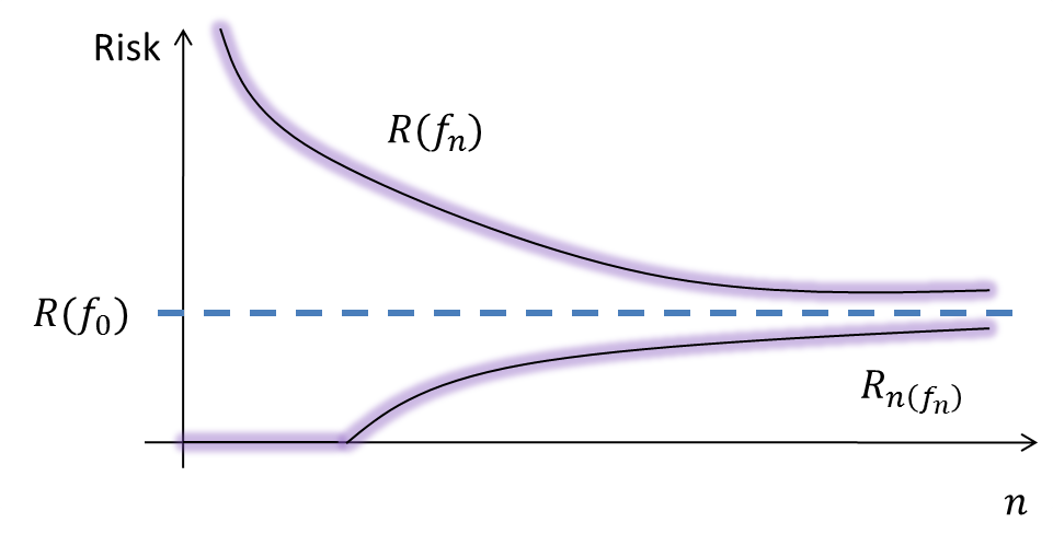
The theoretical curves corresponding to consistent ERM are this:
This can be experimented, for example with SVMs.
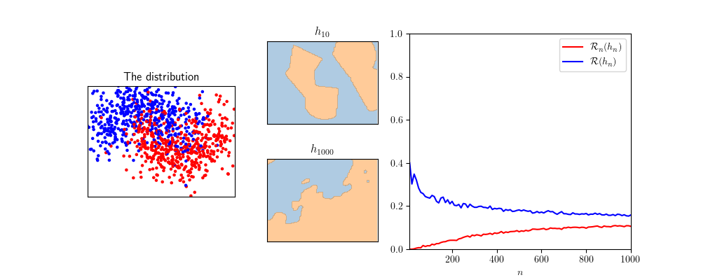
The python source code for such experiments is given below:
import numpy as np
import matplotlib
import matplotlib.pyplot   as plt
import matplotlib.gridspec as gspec
import sklearn.datasets
import sklearn.svm
import sklearn.tree


# We setup the display
matplotlib.rcParams['text.usetex'] = True
xlim = [-1.5, 2.5]
ylim = [-1.5, 1.5]
fig  = plt.figure(figsize=(10,4))
gs   = gspec.GridSpec(2, 3,
                      width_ratios  =[4, 3, 6],
                      height_ratios =[1, 1])

# This function plots the dataset and the decision boundary.
def plot_classifier(classifier, X, y, gridspec, title, draw_contour, draw_samples, Nsamples=100):
    ax = plt.subplot(gridspec)
    ax.set_xlim(xlim)
    ax.set_ylim(ylim)
    ax.set_aspect('equal')
    ax.set_title(title)
    ax.set_xticks([])
    ax.set_yticks([])

    if draw_contour:
        dx = (xlim[1] - xlim[0])/float(Nsamples)
        dy = (ylim[1] - ylim[0])/float(Nsamples)

        xx, yy = np.meshgrid(np.arange(xlim[0], xlim[1], dx),
                             np.arange(ylim[0], ylim[1], dy))
        Z = classifier.predict(np.c_[xx.ravel(), yy.ravel()])
        Z = Z.reshape(xx.shape)
        colors=np.array(['#377eb8','#ff7f00'])
        plt.contourf(xx, yy, Z, alpha=0.4,
                     levels=[0, 0.5, 1.0], colors=colors, zorder=1)

    if draw_samples:
        colors=np.array(['blue','red'])
        plt.scatter(X[:,0], X[:,1], color=colors[y], s=5, zorder=2)

# Ok, here we are ready to do machine learing

# R_n is the measure of the amount of errors made by a classifier on a
# dataset.
def empirical_risk(classifier, X, y) :
    ypred = classifier.predict(X)
    return sum(y != ypred)/float(y.shape[0])

# With artificial distributions (sampler is one such), it is easy to
# generate a new dataset (i.i.d) and to measure the performance of a
# classifier on this dataset. This estimates the real risk (law of
# large numbers), no need for cross-validation here.
def real_risk(classifier, sampler, N=1000) :
    X, y = sampler(N)
    return empirical_risk(classifier, X, y)


# This is the main.

oracle_noise =   0.4  # Set oracle noise (classes get mixed with noise)
Nstep        =    10  # Plot curves every Nstep dataset size.
Nmin         = Nstep  # Min dataset size
Nmax         =  1000  # Max dataset size
nb_average   =    20  # For each n, risks are averaged over nb_average runs.
sampler      = lambda n: sklearn.datasets.make_moons(n, noise=oracle_noise)
experiment   = ['SVM', 'Tree'][2]


if experiment == 'SVM':
    sigma        =    .15  # .05 overfits, 2 has an inductive bias.
    classifier   = sklearn.svm.SVC(C=10,
                                   kernel='rbf', gamma=.5/(sigma*sigma),
                                   tol=1e-5,
                                   decision_function_shape='ovo')
if experiment == 'Tree':
    max_depth    = 100 # Try the parameters, overfitting is not obvious even for deep trees.
    classifier   = sklearn.tree.DecisionTreeClassifier(max_depth         = max_depth,
                                                       min_samples_split = 2)


# Let us plot the learner capabilities
X, y = sampler(Nmax)
plot_classifier(None, X, y, gs[:, 0], 'The distribution', False, True)
X, y = sampler(Nmin)
classifier.fit(X, y)
plot_classifier(classifier, X, y, gs[0, 1], '$h_{{{}}}$'.format(Nmin), True, False)
X, y = sampler(Nmax)
classifier.fit(X, y)
plot_classifier(classifier, X, y, gs[1, 1], '$h_{{{}}}$'.format(Nmax), True, False)

# Let us compute and plot statistics

risks = []
Ns    = [N for N in range(Nmin, Nmax+1, Nstep)]
for N in Ns :
    print('Computing {} risks for N = {}'.format(nb_average, N))
    stats = []
    for k in range(nb_average) :
        X, y = sampler(N)
        classifier.fit(X, y)
        stats.append([empirical_risk(classifier, X, y), real_risk(classifier, sampler, N)])
    risks.append(np.average(np.array(stats), axis=0))
risks = np.array(risks)

ax = plt.subplot(gs[:,2])
ax.set_xlim([Nmin, Nmax])
ax.set_ylim([0, 1])
ax.set_xlabel('$n$')
plt.plot(Ns, risks[:,0], 'r-', label='${{{\\cal R}}}_n(h_n)$')
plt.plot(Ns, risks[:,1], 'b-', label='${{{\\cal R}}}(h_n)$')
plt.legend();

# Show all
plt.savefig('risks.png', layout="tight")
print()
print()
print('risks.png saved')
plt.show()
Hervé Frezza-Buet,