Table of contents

Ensemble Methods (bagging)

Ensemble Methods (bagging)

Introduction

The goal of this lab work is to understand the statistics about functions which are involved in ensemble methods (bagging). First, create a directory for the labwork materials. When you are asked to create or download files, this directory is the place to do it.

Implementation of random variables

From a mathematical point of view, random variables are functions from an event set (for which a probability mesure is defined) to a value set. In our implemantation, a random variable \(X\) is rather considered as a process that can toss values, according to the law of probability \(\mathrm P_X\). A random variable is thus implemented as a function, taking an integer \(n\) as input and computing an n-sized array of outputs.

A random variable whith a uniform distribution in \([0,1]\) is thus the following function:

import numpy as np

def uniform() :
    return lambda nb : np.random.rand(nb)

download the following file randomvar.py.

Read the script. It contain examples which are executed if you run the script:

python3 randomvar.py

Let us get warmed up with a preliminary exercise. Fill the following code…

import randomvar
import numpy as np

def multi_apply(Fs, V) :
   return .....

U = randomvar.uniform()
V = randomvar.apply_array(lambda x : (10*x).astype(int), U)
K = multi_apply([lambda x : x, lambda x : x**2, lambda x : 2*x+1, lambda x : 7*x], V)

randomvar.display(K, 'K')

so that it produces the result below:

mylogin@mymachine:~$ python3 test.py 
K :
  [ 6 36 13 42]
  [1 1 3 7]
  [ 5 25 11 35]
  [1 1 3 7]
  [ 7 49 15 49]
  [ 6 36 13 42]
  [0 0 1 0]
  [ 4 16  9 28]
  [1 1 3 7]
  [1 1 3 7]

Once done, check your answer (file warm-up.py).

Interface with scikit

In scikit-learn, dataset are provided as a pair of vectors \((x,y)\). In our experiment, we will rather consider a list of triplets \((x_x, x_y, y)\). Moreover, in order to fit the mathematics, we need to handle predictors as functions, provided by a fitted classifier.

Download and read ml.py. Test the following code.

import sklearn.datasets
import numpy as np
import ml

Z = lambda n: ml.S_from_sklearn(sklearn.datasets.make_circles(n, noise=0.1, factor=0.75))
S = Z(10) # let us make a dataset from the random variable Z
print(S)
print(ml.x_of(S))
print(ml.y_of(S))
X, y = ml.S_to_sklearn(S)
print(X)
print(y)

In our experiments, we will use the moons dataset provided by scikit as a \(Z\) variable. Since it is not purely i.i.d in the scikit implementation (especially for small datasets), what has been done previously for the circle dataset cannot be applied for moons directly. Thus, let us add a moons \(Z\) random variable in ml.py.

import sklearn.datasets

def Z_moons(n) :
    noise = .2
    if n > 100 :
        return S_from_sklearn(sklearn.datasets.make_moons(n, noise=noise))
    else:
        S = S_from_sklearn(sklearn.datasets.make_moons(1000, noise=noise))
        np.random.shuffle(S)
        return S[0:n]

Last, we will need a good and a bad (i.e. overfitting) classifier to test things in incoming exercises. Let us use C-SVCs for both. The detail of SVMs is out of the scope of the present lab work. Here, just add in the ml.py file the following definitions:

import sklearn.svm

def overfitting_classifier() :
    return sklearn.svm.SVC(C=100, kernel='rbf', gamma = 20)

def good_classifier() :
    return sklearn.svm.SVC(C=100, kernel='rbf', gamma = .5)

The SVC classifier has a method fit and a method predict, as most algorithms in sklearn. To train such a classifier, we would do the following:

S = Z_moons(50) # Learning set
T = Z_moons(50) # Test set
classifier = overfitting_classifier()
X, y = ml.S_to_sklearn(S)
classifier.fit(X, y)                    # Learning is done here
y_pred = classifier.predict(ml.x_of(T)) # Here, we use what we have learnt

Matplotlib drawings

We consider in these exercises the data as realizations of a random variable \(Z = (X,Y) \in \left([a,b]\times[c,d] \right) \times \left\{0, 1\right\}\). The values \((a,b)\) and \((c,d)\) are denoted by xbounds and ybounds respectively. Drawings are implemented in draw.py, download and read this file and test the following code.

import matplotlib.pyplot as plt
import sklearn.datasets
import numpy as np
import ml
import draw

Z = lambda n: ml.S_from_sklearn(sklearn.datasets.make_circles(n, noise=0.1, factor=0.75))
S = Z(100) # let us make a dataset from the random variable Z
h = lambda X : (X[:,0]**2 + X[:,1]**2 < 1).astype(int)

plt.figure(figsize = (10,5))
xbounds = (-2, 2)
ybounds = (-2, 2)

ax = plt.subplot(1, 2, 1)
draw.no_tics(ax)
draw.decision_boundary_2d(ax, h, xbounds, ybounds)
draw.samples_2d(ax, S)

ax = plt.subplot(1, 2, 2)
draw.no_tics(ax)
draw.decision_boundary_2d(ax, h, xbounds, ybounds)
draw.prediction_2d(ax, h, ml.x_of(S))

plt.show()

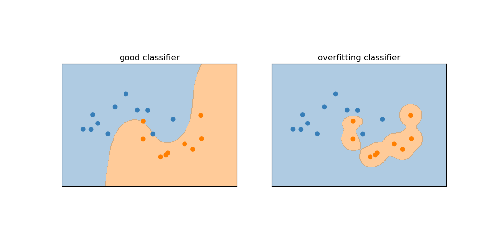
Write a short python script, involving functions defined in both ml.py and draw.py files, to plot a figure like the one below. Do not forget to use ml.Z_moons and ml.predictor.

Statistical learning implementation

Let us add functions in ml.py in order to implement basic machine learning concepts.

Real risk

The real risk of a hypothesis \(h\) is defined as the expectancy of the random variable \(l(h(X),Y)\), where \(l(y,y')\) is the loss function.

\[R(h) = \mathrm E(l(h(X), Y)),\; Z = (X,Y)\]

Making the hypothesis that the implementation of \(h\) enables to pass an array of input as argument (as results of ml.predictor), implement in ml.py a function for computing the real risk. To do so, you are invited to use the randomvar.expectancy and randomvar.apply_array functions implemented in randomvar.py. Test the function by running the following code:

import sklearn.datasets
import numpy as np
import ml

Z = lambda n: ml.S_from_sklearn(sklearn.datasets.make_circles(n, noise=0.1, factor=0.75))
h = lambda X: (X[:,0]**2 + X[:,1]**2 < 1).astype(int)
loss = lambda y1, y2: y1 != y2

# expectancy is estimated from 10000 samples.
R = ml.real_risk(h, loss, Z, 10000)
print('R(h) = {} close to 0.24'.format(R))

Learning

In the statistical learning theory, the hypothesis \(h_n\) is the predictor obtained when we fit a dataset \(D\). As the dataset is a random variable as well (it is indeed a n-uplet of \(Z\) random variables), the expression \(h_n\) is a random variable (i.e. a random function). Add a function fit in ml.py implementing the random variable \(h_n\). As fitting data may raise an exception (if there is only one class in the data), use randomvar.apply_retry rather than randomvar.apply for implementing fit.

If you write erroneous code (bad syntax, wrong variable name; …), python raises an exception at runtime. So randomvar.apply_retry will retry until your code raises no exception… this never occurs of course since the code do not get corrected by itself, your execution thus loops forever. So at first, use randomvar.apply and switch to randomvar.apply_retry when you are out of syntactical issues.

The following code

import matplotlib.pyplot as plt
import numpy as np
import ml
import randomvar
import draw

Z = ml.Z_moons
D = randomvar.nuplet(Z, 20)
h_n = ml.fit(ml.good_classifier, D)

plt.figure(figsize = (10, 10))
xbounds = (-2, 3)
ybounds = (-1.5, 2)
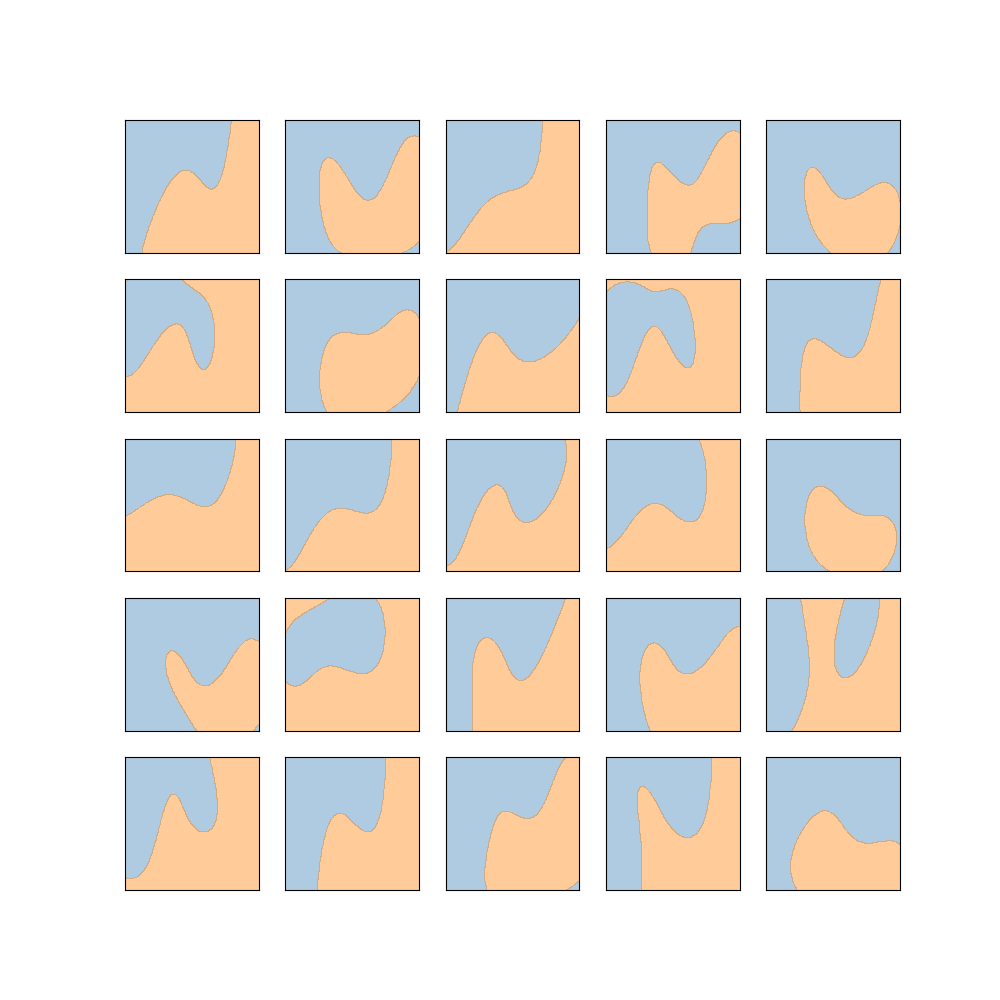
for i, h in enumerate(h_n(25)):
    ax = plt.subplot(5, 5, i+1)
    draw.no_tics(ax)
    draw.decision_boundary_2d(ax, h, xbounds, ybounds, Nsamples=200)
plt.show()

should plot something like

Functional and statistical difference

The previous figure shows that functions vary one from the other. In order to measure such variations, we will compute a functional difference between two functions. We will give this difference a problem-related statistical flavor (the problem in question is \(Z\)). Let us define the difference between two hypotheses as:

\[h - h' = \mathrm E (l(h(X), h'(X))),\; Z = (X,Y)\]

In the file ml.py, add a function diff such as the follwing code

import matplotlib.pyplot as plt
import ml
import draw
import randomvar

Z = ml.Z_moons
S = Z(100)
D = randomvar.nuplet(Z, 20)
h_n = ml.fit(ml.good_classifier, D)
loss = lambda y1, y2 : y1 != y2
N = 1000 # for expectancy estimation

h1, h2 = h_n(2)
h3 = lambda X, f=h1, g=h2: loss(f(X), g(X))

plt.figure(figsize = (9, 3))
xbounds = (-2, 3)
ybounds = (-1.5, 2)

ax = plt.subplot(1, 3, 1)
draw.no_tics(ax)
draw.decision_boundary_2d(ax, h1, xbounds, ybounds, Nsamples=200)

ax = plt.subplot(1, 3, 2)
draw.no_tics(ax)
draw.decision_boundary_2d(ax, h2, xbounds, ybounds, Nsamples=200)

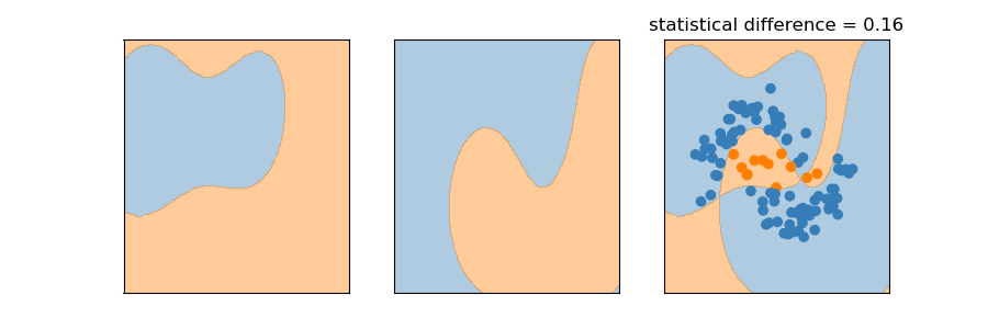
ax = plt.subplot(1, 3, 3)
ax.set_title('statistical difference = {}'.format(ml.diff(h1, h2, loss, Z, N)))
draw.no_tics(ax)
draw.decision_boundary_2d(ax, h3, xbounds, ybounds, Nsamples=200)
draw.prediction_2d(ax, h3, ml.x_of(S))

plt.show()

plot something like

Bagging

Functional tools

Download the functional.py file in your working directory. Read the code.

Aggregating

Consider the moons dataset random variable \(D\) of size \(n\) (using randomvar.nuplet as previously), a functional random variable \(h_n\) built from it with the ml.overfitting_classifier algorithm. With randomvar.nuplet, define a random variable \(H_{n,k} = (h^1, h^2, \cdots, h^k)\) that is a \(k\)-uplet of functional random variables, such as all \(h^i\) follows the same law as \(h_n\) and are independent. Then, using randomvar.apply and functional.majority_merge, implement a random variable \(a_{n,k}\) corresponding to the random aggregation of the \(k\) functions.

Plot a realization of \(h_n\) and \(a_{n,k}\), in order to get the following plot (with \(n=20\), \(k=10\)).

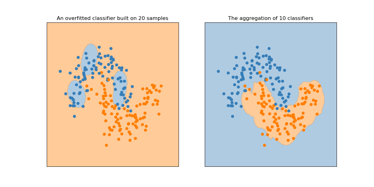
You can first generate a dataset \(S\) and and then built the dataset random variable \(D\) from randomvar.bootstrap. This simple changes makes the whole process a Bagging process. This is investigated further.

Variance analysis

For scalar random variables, the variance is expressed as

\[\mathrm{var}(X) = \mathrm E \left( X - \mathrm E (X) \right) ^2\]

Here, instead of \(X\), let us rather consider a random function \(a_{n,k}\). Let us fix \(n=10\).

As a warming up, plot the values \(a - a'\) where random variables \(a\) and \(a'\) are the same random variable \(a_{n,k}\), for increasing values of \(k\). The difference \(a-a'\) here is the functional and statistical difference introduced previously. For each k, you can plot a bunch of 50 differences, as well as the mean and the standard deviation of them.

Now we can plot what is similar to a functional standard deviation of \(h_n\). Indeed, this is \(\mathrm E \left( h_n - \mathrm E \left(h_n\right)\right) = \mathrm E \left(h_n - a_{n,K}\right)\). The expression \(a_{n,K}\) stands for \(\mathrm E \left(h_n\right)\), if we take a big K. (choose \(K = 50\) for example, or greater if you can afford the computation). Show experimentally the influence of \(n\).

For \(n=10\), compare the standard deviation of \(h_n\), as previously defined, with the standard deviation of \(a_{n,k}\). The expectancy \(\mathrm E \left(a_{n,k}\right)\) needs to be estimated as well, as we did for \(\mathrm E \left(h_n\right)\) previously.

Bootstrapping

With the moons dataset, we can afford sampling as many value as we need. This is not the case in most real machine learning situations. This is where bootstrapping gets involved.

Consider now a dataset \(S\) of size \(N\), obtained from the moons distribution. Do the same study as previously, with the random variable \(D\) being obtained by bootstrapping from \(S\). You can chose \(N = n = 20\). The datasets generated by \(D\), and thus the \(H_{n,k}\), are not independent anymore.

Plot the variance reduction obtained from bootstrapping and compare to the pevious case. You should notice less reduction with bootstrapping.

Playing with trees

Bootstrapping is rather used with deep decision trees (i.e. split until leaves have all the same label, such trees may overfit). From the tools developped so far, implement a study of the influence of bootstrapping on the variance with such decision trees.

When you’re done

Here is an example of what could have been done. See Corrige-TP-Ensembles.tar.gz.

Hervé Frezza-Buet,