The CxSOM experiments

In the cxsom-builder package, there are examples named “example-xxx-yyy-experiment”. When you install the package, they provide an executable that can be used to set up experiments.

An experiment consists in using the cxsom tools to fully analyse some architecture. In the “experiment” section of the cxsom-builder package, all the customized pieces of code for running such an analyze, for a given experiment, are provided, as an example of what can be done with cxsom.

All the computation for an experiment is managed by a specific makefile, consider it as an example as well.

In one of the experiments directory, you will find a readme file, that gives you instructions to conduct the experiment by yourself.

Experiment 003-001, the X/Y maps.

This experiment is the basic one, when two maps are connected together. Each map is fed with one coordinate of the points belonging to a curve in the plan.

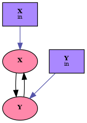
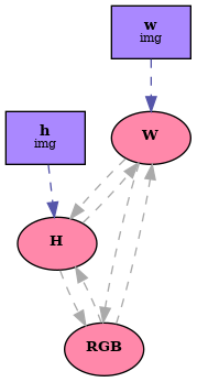
The cxsom-builder architecture notation. — The `cxsom-builder` architecture notation.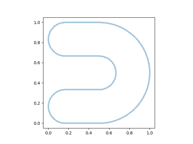

The experiment leads to the generation of a movie, where the self-organization is illustrated. We feed the architecture with 2500 samples (i.e. there are 2500 timesteps). We make statistics for building one frame of the movie at every five timesteps.

Experiment 003-002, color prediction with W/H/RGB maps.

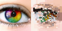
In this experiment, we consider the image below as a function. Indeed, it can be viewed as a mapping of \((w, h) \in {[0, 1]}^2\) onto \(\mathrm{rgb} \in {[0, 1]}^3\), where \((w, h)\) is the coordinates of the pixels and \(\mathrm{rgb}\) their color.

The experiments consists in using 3 maps, 1D, one for \(w\), one for \(h\) and one for \(\mathrm{rgb}\), connect them together and feeding the with randomly choosen pixels \((w, h, \mathrm{rgb})\) (see the rules).

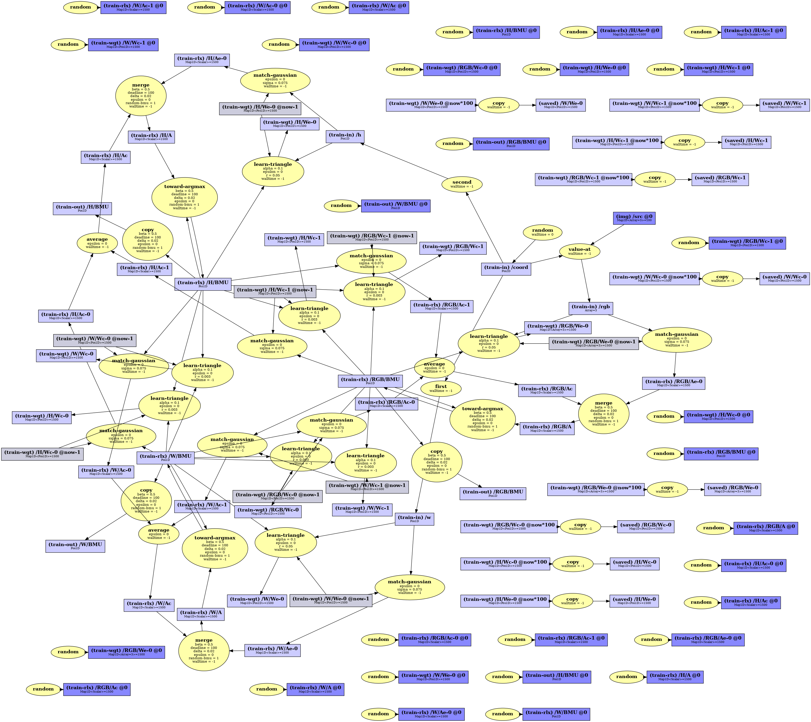
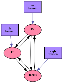
The cxsom-builder training architecture notation. — The `cxsom-builder` training architecture notation.

Then, we used the trained weights, but remove the \(\mathrm{rgb}\) inputs. We submit \((w, h)\) pixels spanning uniformly \({[0, 1]}^2\), let the architecture relax and find a BMUs in each maps, and use the external weights in the map handling \(\mathrm{rgb}\) values as a look-up table, providing a color for the BMU found in the \(\mathrm{rgb}\)-map (see the rules).

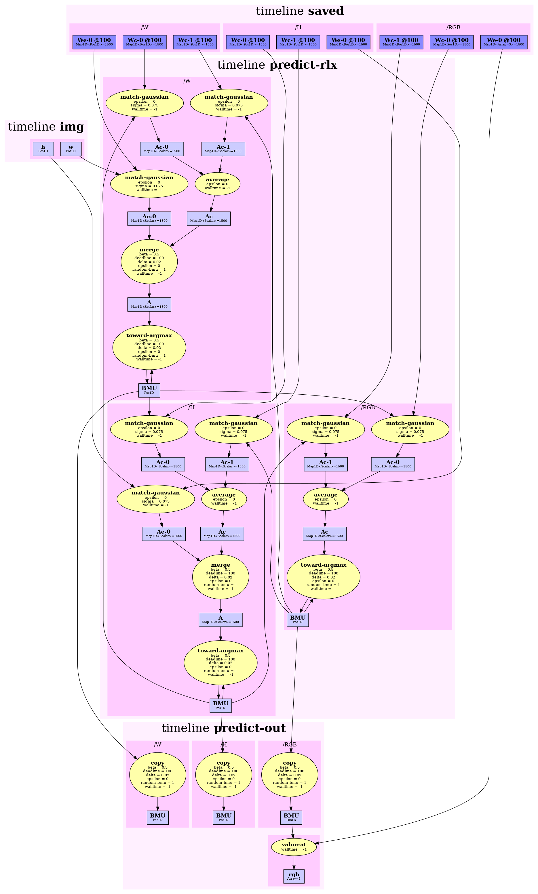
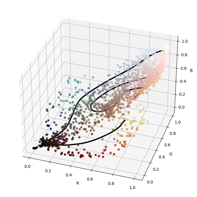
The cxsom-builder predicting architecture notation. — The `cxsom-builder` predicting architecture notation.

This is the reconstruction obtaines after training on 30000 samples.

The external weights in the RGB map forms a 1D path in the 3D RGB space.

External weight final organization in the RGB map.

Let us see how things evolve.

Every 100 steps (i.e. 100 samples provided for training), we display the reconstruction (i.e. the prediction, on the right) and the fitting. The fitting is obtained by feeding the architectures with \((w, h)\) pixels spanning uniformly \({[0, 1]}^2\), as for prediction, but also providing the corresponding \(\mathrm{rgb}\) value, as for training. The architecture then uses these 3 inputs to relax, and we display the weight values at each BMU in each map. This leads to pixels \((w, h, \mathrm{rgb})\), shown on the left figure in the movie. Many pixel positions overlap on few positions, so the whole patch \({[0, 1]}^2\) is not represented, whereas the actual \((x, h)\) inputs cover it uniformly.

The weights evolves as follows

Hervé Frezza-Buet,