License : Creative Commons Attribution 4.0 International (CC BY-NC-SA 4.0)
Copyright :
Hervé Frezza-Buet,
CentraleSupelec
Last modified : March 28, 2024 13:08
Link to the source : som.md
Implementing a basic SOM with CxSOM
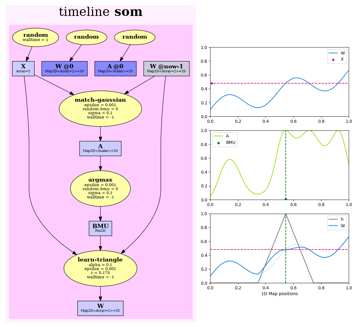
Let us enter into cxsom with the implementation of a basic 2D SOM, handling 2D samples.
The SOM algorithm expressed in CxSOM
Mathematical formulation
The inputs are \(X^t \in {[0, 1]}^2\), and we project them into a \(20\times20\) grid of prototypes. Each prototype is denoted by \(W_{ij} \in {[0, 1]}^2, (i,j) \in \{1, \ldots, 20\}^2\), and its value at time \(t\) is denoted by \(W_{ij}^t\).
Matching an input \(X^t\) against each prototype in the map \(W^{t-1}\) leads to a map of matching values
\(\forall (i,j), \; A_{ij}^t \in [0,1] = \mu(X^t, W_{ij}^{t-1}) = \exp\left(-\frac{\left\| X^t- W_{ij}^{t-1} \right\|^2}{2\sigma^2}\right)\)
The best matching unit \(\mathrm{BMU}^t\) is the the \((i,j)\) coordinates of the highest \(A_{ij}^t\).
The whole weights are then updated, according to to that \(\mathrm{BMU}^t\) (i.e. the ones around that position), in order to get closer to \(X^t\). This can be written as
\(W^t = \mathrm{learn}(W^{t-1}, \mathrm{BMU}^t, X^t)\)
i.e,
\(\forall (i,j),\; \alpha'_{ij} = \alpha h\left(\left\|\mathrm{BMU}^t - (i,j)\right\|\right),\; W_{ij}^t = (1-\alpha'_{ij})W_{ij}^{t-1} + \alpha'_{ij}X^t\)
The value \(W^0\) and \(A^0\) can be set randomly for the first step \(t=0\), but then, the general updating scheme described so far applies. Let us also compute \(X^t\) as a random value at any time.
This is what the following picture shows:
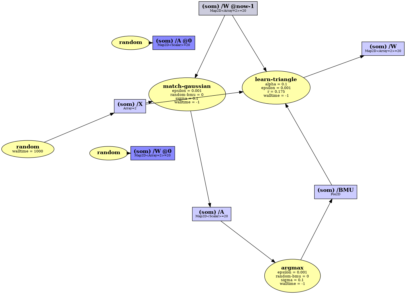
The CxSOM formulation
Indeed, cxsom enables you to describe those rules in a C++ file. This is what it looks like.
// This is the som.cpp file, describing the SOM updating rules.

#include <cxsom-rules.hpp>
using namespace cxsom::rules;
context* cxsom::rules::ctx = nullptr;

#define CACHE         2 // nb of instances kept in processor memory
#define WTRACE   100000 // Size of the weight buffer
#define XTRACE    10000 // Size of the input buffer
#define FORGET        0 // Size of the 0-sized buffers.
#define OPENED     true // We keep the files opened at processor side.
#define XWALLTIME  1000 // The random input rule dies after that time.

int main(int argc, char* argv[]) {
  context c(argc, argv);

  kwd::parameters p_main, p_match, p_learn;
  p_main  |         kwd::use("walltime", -1), kwd::use("epsilon",    1e-3 );
  p_match | p_main, kwd::use("sigma",    .1), kwd::use("random-bmu", 0    );
  p_learn | p_main, kwd::use("alpha",    .1), kwd::use("r",          0.175);

  {
    timeline t("som");

    kwd::type("X",   "Array=2",           CACHE, XTRACE, OPENED);
    kwd::type("W",   "Map2D<Array=2>=20", CACHE, WTRACE, OPENED);
    kwd::type("A",   "Map2D<Scalar>=20",  CACHE, FORGET, OPENED);
    kwd::type("BMU", "Pos2D",             CACHE, FORGET, OPENED);

    kwd::at("W", 0) << fx::random();
    kwd::at("A", 0) << fx::random();

    "X"   << fx::random()                                   | kwd::use("walltime", XWALLTIME);
    "A"   << fx::match_gaussian("X", kwd::prev("W"))        | p_match;
    "BMU" << fx::argmax("A")                                | p_match;
    "W"   << fx::learn_triangle("X", kwd::prev("W"), "BMU") | p_learn;
  }

  return 0;
}
This code can be compiled by the command
mylogin@mymachine:~$ g++ -o som -std=c++17 som.cpp $(pkg-config --cflags --libs cxsom-rules)
The som executable can be used for several purposes. Among them, it can generate the figure displayed in the previous section thanks to graphviz:
mylogin@mymachine:~$ ./som graph fig
mylogin@mymachine:~$ dot -Tpdf fig-updates.dot -o figure.pdf
For some more complex update schemes, other graph layout may be easier to read. For our simple SOM, it can be produced like this.
mylogin@mymachine:~$ ./som graph-full ffig
mylogin@mymachine:~$ sfdp -Tpdf -Goverlap=prism ffig-updates.dot -o ffigure.pdf
The argument graph-full adds the timeline name and the full variable path to the variable graph node names. You get this, thanks to graphviz as well.
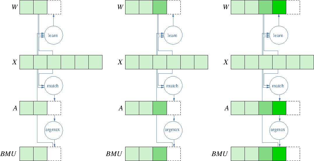
The CxSOM execution
Each square in the figure below is a “data instance” (DI), i.e. the value of a variable at some instant. Updates described by rules aim at computing new DIs as soon as update operands are available. Applying updates (in parallel) is the cxsom computation, made by the cxsom-processor
Running the SOM simulation
Execution
First, you have to define where the files will be stored. This workspace is names a “root dir”, let us call it root_dir in the following. Let us create this directory first.
mylogin@mymachine:~$ mkdir root_dir
Starting a simulation consists of running a “cxsom processor”, 4 is the number of threads that we will use, and 10000 is the port on which the processor will listen for queries. Let us create and use a makefile in order to activate those elements in a convenient way.
mylogin@mymachine:~$ echo include /usr/share/cxsom/cxsom-makefile > Makefile
mylogin@mymachine:~$ make
Now we configure our project.
mylogin@mymachine:~$ make cxsom-set-config ROOT_DIR=./root_dir HOSTNAME=localhost PORT=10000 NB_THREADS=4
mylogin@mymachine:~$ make cxsom-show-config
Let us start on the current machine (this is why we used localhost as HOSTNAME) the processor that will execute updates for us.
mylogin@mymachine:~$ make cxsom-launch-processor
mylogin@mymachine:~$ make cxsom-is-processor-running
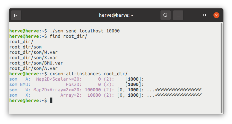
Last, let us inspect the directory where our variables will be written. It is empty, but keep the opened terminal alive for the next stages.
mylogin@mymachine:~$ make cxsom-scan-vars
You can use the som executable compiled previously to send the updating rules to the processor. We remind you with the compiling line and then we send the rules (to localhost here, in the case of a processor running on the same machine).
mylogin@mymachine:~$ g++ -o som -std=c++17 som.cpp $(pkg-config --cflags --libs cxsom-rules)
mylogin@mymachine:~$ ./som send localhost 10000
And that’s it !
Some tools enable you to see what is currently computed by the processor, but these are more easy when called from the makefile once configuration is done.
Feeding
The pycxsom library enables to write the manipulation of the files in root_dir. Let us illustrate this by writing a script feed.py that feeds our SOM with new inputs.
# file feed.py

import os
import sys
import pycxsom as cx
import numpy as np

if len(sys.argv) < 3:
    print()
    print('Usage:')
    print('  {} [crown|square|triangle] <root_dir> [<hostname> <port>]'.format(sys.argv[0]))
    print()
    sys.exit(0)

distrib   = sys.argv[1]
root_dir  = sys.argv[2]

nb_to_send = 5000 # We send a bunch of samples of that size.

# We access to the data file <rootdir>/som/X.var
with cx.variable.Realize(cx.variable.path_from(root_dir, 'som', 'X')) as xi:
    while nb_to_send > 0: # We may produce less than nb_to_send samples at each iteration.
        Xs = np.random.rand(nb_to_send)
        Ys = np.random.rand(nb_to_send)
        if distrib == 'crown':
            rmin, rmax = .35, .5
            R2s = (Xs - .5)**2 + (Ys - .5)**2
            keep = np.logical_and(rmin**2 < R2s, R2s < rmax**2)
            Xs, Ys = Xs[keep], Ys[keep]
        elif distrib == 'triangle':
            keep = Xs > Ys
            Xs, Ys = Xs[keep], Ys[keep]
        elif distrib == 'square':
            pass
        else:
            print()
            print()
            print('Distribution {} is invalid'.format(distrib))
            print()
            sys.exit(0)

        if len(Xs) > nb_to_send :
            sent = nb_to_send
            Xs, Ys = Xs[:nb_to_send], Ys[:nb_to_send]
        else:
            sent = len(Xs)

        # We format the data as [[x, y], [x, y], ....]
        XYs = np.stack((Xs, Ys)).T
        # Each line is a [x, y] that we add to the xi file.
        for xy in XYs: xi += xy

        nb_to_send -= sent

# We tell the server to wake up since we have added new data that should
# unlock computation.
if len(sys.argv) == 5:
    hostname  = sys.argv[3]
    port      = int(sys.argv[4])
    print('Sending "ping" to {}:{}'.format(hostname, port))
    if cx.client.ping(hostname, port):
        print('Something went wrong.')
It can be executed several times, feeding with examples tossed from different shapes.
mylogin@mymachine:~$ python3 feed.py square root_dir/ localhost 10000
mylogin@mymachine:~$ python3 feed.py crown root_dir/ localhost 10000
mylogin@mymachine:~$ python3 feed.py triangle root_dir/ localhost 10000
The processor, as soon as new data is available, continues the execution of the updating rules.
Viewing
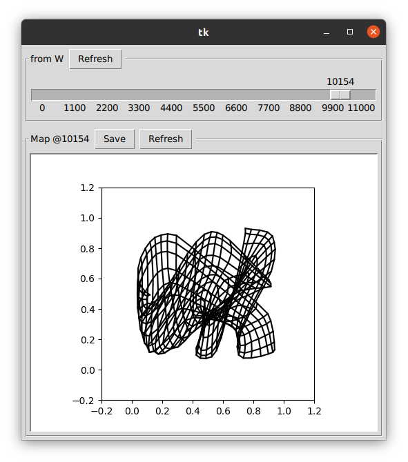
The pycxsom library enables to write nice viewers as well. Let us implement a viewer visu.py for displaying the weights evolution.
# file visu.py

import sys
import pycxsom as cx
import numpy as np
import tkinter as tk
import matplotlib as plt


if len(sys.argv) != 2:
    print()
    print('Usage:')
    print('  {} <rootdir>'.format(sys.argv[0]))
    print()
    sys.exit(0)

root_dir = sys.argv[1]
w_path   = cx.variable.path_from(root_dir, 'som', 'W') # W is <rootdir>/som/W.var

# This is a cxsom tool for viewing with matplotlib.
class MapViewer(cx.tkviewer.At):
    def __init__(self, master, title, figsize=(5, 4), dpi=100):
        super().__init__(master, title, figsize, dpi)

    def on_draw_at(self, at):
        self.fig.clear()    # self.fig is the matplotlib figure
        ax = self.fig.gca()
        ax.set_aspect('equal')
        ax.set_xlim(-.2, 1.2)
        ax.set_ylim(-.2, 1.2)
        with cx.variable.Realize(w_path) as var:
            W = var[at]
            Wx, Wy = W[...,0], W[...,1]
            for X, Y in zip(Wx,   Wy  ): ax.plot(X, Y, 'k') # These two lines...
            for X, Y in zip(Wx.T, Wy.T): ax.plot(X, Y, 'k') # ... draw the grid.

# We open a GUI main window.
root = tk.Tk()
root.protocol('WM_DELETE_WINDOW', lambda : sys.exit(0))

# We add a slider synchronized with the instants stored in our W variable.
slider = cx.tkviewer.HistoryFromVariableSlider(root, 'from W', w_path)
slider.widget().pack(fill=tk.BOTH, side=tk.TOP)

# We add our viewer...
viewer = MapViewer(root, 'Map')
viewer.widget().pack(fill=tk.BOTH, side=tk.TOP)
viewer.set_history_slider(slider) # ... telling to draw the instant got from the slider.

# Then we start the GUI.
tk.mainloop()
mylogin@mymachine:~$ python3 visu.py root_dir/
This is how it looks like.
Restart from a saved state
Let us kill the server.
mylogin@mymachine:~$ make cxsom-kill-processor
All the computed values are saved in the files written on your root_dir. You can still visualize them, feed new data.
mylogin@mymachine:~$ python3 feed.py square root_dir/
In order to restart from a previously saved state, you just need to restart a processor,
mylogin@mymachine:~$ make cxsom-launch-processor
and re-send the updating rules to it.
mylogin@mymachine:~$ ./som send localhost 10000
It will continue from updates to be done according to the data in the files.
Debugging
The simulation stops when nothing more can be computed, usually because none of the possible updates have all their required entries available.
In case of an unexpected blocking, you may need to investigate the reasons. To do so, cxsom provides you with debugging tools.
Expert debugging (verbose processor)
This is rather reserved to developpers. The idea is to launch a verbose cxsom processor, and analyse the output on the terminal.
mylogin@mymachine:~$ make cxsom-launch-verbose-processor
and then send rules, as previously.
User friendly debugging (monitored processor)
The idea is to launch a monitored processor, it feeds a text file which describes, line by line, what happens. The grammar of this text file is specified is the source file cxsomLog.hpp, as a comment, but is can be easier to use a python parser to read this file.
Let us illustrate this with an example, restarting from scratch.
mylogin@mymachine:~$ make cxsom-kill-processor
mylogin@mymachine:~$ make cxsom-clear-rootdir
mylogin@mymachine:~$ make cxsom-scan-vars
mylogin@mymachine:~$ make cxsom-launch-monitored-processor
Now let us compute some few steps.
mylogin@mymachine:~$ ./som send localhost 10000
mylogin@mymachine:~$ python3 feed.py square root_dir/ localhost 10000
Reading the monitoring data file
Let us have a look to the generated file monitoring.data. Each line is something done (and reported) by the processor. Some lines are like # 201, i.e # followed by an integer (increasing). These lines are checkpoints in the file. Each time a new computation is attempted, a new checkpoint appears in the file.
As previously said, reading this file may be easier with python, using the script interactivly.
mylogin@mymachine:~$ python3
Then type the following lines one by one in the python shell.
from pycxsom.monitor import Monitor
m = Monitor()
# m enables to parse the monitor.data file

len(m)
# this tells you how many chekpoints are available in the file.

m.goto(10)   # goto checkpoint 10
m.position() # returns 10
m += 3       # skip forward 3 checkpoints
m.position() # returns 13
m.goto()
m.position() # return 0

# Once you get positionned at some checkpoint, you can parse the lines one after the other, and get a json-like data as a result at each call.

m.goto(10)
next(m) # returns: {'type': 'job', 'info': 'tasks', 'tasks': [{'timeline': 'som', 'var': 'W', 'at': 1}]}
next(m) # returns: {'type': 'job', 'info': 'execute', 'task': {'timeline': 'som', 'var': 'BMU', 'at': 1}}
next(m) # returns: {'type': 'timestep', 'info': 'report', 'timestep': {'timeline': 'som', 'at': 1}, 'var': 'BMU', 'status': 'done'}
next(m) # returns: {'type': 'timestep', 'info': 'update', 'timestep': {'timeline': 'som', 'at': 1}, 'why': 'notification', 'status': 'relaxing', 'new': [], 'unstable': ['W'], 'impossible': [], 'stable': [], 'confirmed': [], 'blockers': []}
next(m) # returns: {'type': 'checkpoint', 'info': 11}

next(m) # returns: {'type': 'job', 'info': 'tasks', 'tasks': []}

next(m) # returns: {'type': 'job', 'info': 'execute', 'task': {'timeline': 'som', 'var': 'W', 'at': 1}}
# ...
Using the monitor datafile to generate a situation report
When the computation is blocked, if you wonder why, you can launch the following tool.
mylogin@mymachine:~$ make cxsom-monitoring-report
This tool reads the current version of monotoring.data and generates/overwrite the file monitoring.md. This is a markdown file. To permanently display the current version of it, you can launch on another terminal
mylogin@mymachine:~$ grip monitoring.md
and view the webpage suggested by grip on a navigator. You may get something like this
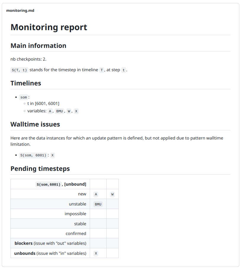
monitoring.md with the command grip.